Equalities that involve trigonometric functions
Trigonometry Functions (sin, cos, tan, inverse) Generalized trigonometry Reference Identities Exact constants Tables Unit circle Laws and theorems Sines Cosines Tangents Cotangents Calculus Mathematicians
In trigonometry , trigonometric identities are equalities that involve trigonometric functions and are true for every value of the occurring variables for which both sides of the equality are defined. Geometrically, these are identities involving certain functions of one or more angles . They are distinct from triangle identities , which are identities potentially involving angles but also involving side lengths or other lengths of a triangle .
These identities are useful whenever expressions involving trigonometric functions need to be simplified. An important application is the integration of non-trigonometric functions: a common technique involves first using the substitution rule with a trigonometric function , and then simplifying the resulting integral with a trigonometric identity.
Pythagorean identities Trigonometric functions and their reciprocals on the unit circle. All of the right-angled triangles are similar, i.e. the ratios between their corresponding sides are the same. For sin, cos and tan the unit-length radius forms the hypotenuse of the triangle that defines them. The reciprocal identities arise as ratios of sides in the triangles where this unit line is no longer the hypotenuse. The triangle shaded blue illustrates the identity 1 + cot 2 θ = csc 2 θ {\displaystyle 1+\cot ^{2}\theta =\csc ^{2}\theta } tan 2 θ + 1 = sec 2 θ {\displaystyle \tan ^{2}\theta +1=\sec ^{2}\theta } The basic relationship between the sine and cosine is given by the Pythagorean identity:
sin 2 θ + cos 2 θ = 1 , {\displaystyle \sin ^{2}\theta +\cos ^{2}\theta =1,} where sin 2 θ {\displaystyle \sin ^{2}\theta } ( sin θ ) 2 {\displaystyle (\sin \theta )^{2}} cos 2 θ {\displaystyle \cos ^{2}\theta } ( cos θ ) 2 . {\displaystyle (\cos \theta )^{2}.}
This can be viewed as a version of the Pythagorean theorem , and follows from the equation x 2 + y 2 = 1 {\displaystyle x^{2}+y^{2}=1} unit circle . This equation can be solved for either the sine or the cosine:
sin θ = ± 1 − cos 2 θ , cos θ = ± 1 − sin 2 θ . {\displaystyle {\begin{aligned}\sin \theta &=\pm {\sqrt {1-\cos ^{2}\theta }},\\\cos \theta &=\pm {\sqrt {1-\sin ^{2}\theta }}.\end{aligned}}} where the sign depends on the quadrant of θ . {\displaystyle \theta .}
Dividing this identity by sin 2 θ {\displaystyle \sin ^{2}\theta } cos 2 θ {\displaystyle \cos ^{2}\theta }
1 + cot 2 θ = csc 2 θ 1 + tan 2 θ = sec 2 θ sec 2 θ + csc 2 θ = sec 2 θ csc 2 θ {\displaystyle {\begin{aligned}&1+\cot ^{2}\theta =\csc ^{2}\theta \\&1+\tan ^{2}\theta =\sec ^{2}\theta \\&\sec ^{2}\theta +\csc ^{2}\theta =\sec ^{2}\theta \csc ^{2}\theta \end{aligned}}} Using these identities, it is possible to express any trigonometric function in terms of any other (up to a plus or minus sign):
Each trigonometric function in terms of each of the other five.[1] in terms of sin θ {\displaystyle \sin \theta } csc θ {\displaystyle \csc \theta } cos θ {\displaystyle \cos \theta } sec θ {\displaystyle \sec \theta } tan θ {\displaystyle \tan \theta } cot θ {\displaystyle \cot \theta } sin θ = {\displaystyle \sin \theta =} sin θ {\displaystyle \sin \theta } 1 csc θ {\displaystyle {\frac {1}{\csc \theta }}} ± 1 − cos 2 θ {\displaystyle \pm {\sqrt {1-\cos ^{2}\theta }}} ± sec 2 θ − 1 sec θ {\displaystyle \pm {\frac {\sqrt {\sec ^{2}\theta -1}}{\sec \theta }}} ± tan θ 1 + tan 2 θ {\displaystyle \pm {\frac {\tan \theta }{\sqrt {1+\tan ^{2}\theta }}}} ± 1 1 + cot 2 θ {\displaystyle \pm {\frac {1}{\sqrt {1+\cot ^{2}\theta }}}} csc θ = {\displaystyle \csc \theta =} 1 sin θ {\displaystyle {\frac {1}{\sin \theta }}} csc θ {\displaystyle \csc \theta } ± 1 1 − cos 2 θ {\displaystyle \pm {\frac {1}{\sqrt {1-\cos ^{2}\theta }}}} ± sec θ sec 2 θ − 1 {\displaystyle \pm {\frac {\sec \theta }{\sqrt {\sec ^{2}\theta -1}}}} ± 1 + tan 2 θ tan θ {\displaystyle \pm {\frac {\sqrt {1+\tan ^{2}\theta }}{\tan \theta }}} ± 1 + cot 2 θ {\displaystyle \pm {\sqrt {1+\cot ^{2}\theta }}} cos θ = {\displaystyle \cos \theta =} ± 1 − sin 2 θ {\displaystyle \pm {\sqrt {1-\sin ^{2}\theta }}} ± csc 2 θ − 1 csc θ {\displaystyle \pm {\frac {\sqrt {\csc ^{2}\theta -1}}{\csc \theta }}} cos θ {\displaystyle \cos \theta } 1 sec θ {\displaystyle {\frac {1}{\sec \theta }}} ± 1 1 + tan 2 θ {\displaystyle \pm {\frac {1}{\sqrt {1+\tan ^{2}\theta }}}} ± cot θ 1 + cot 2 θ {\displaystyle \pm {\frac {\cot \theta }{\sqrt {1+\cot ^{2}\theta }}}} sec θ = {\displaystyle \sec \theta =} ± 1 1 − sin 2 θ {\displaystyle \pm {\frac {1}{\sqrt {1-\sin ^{2}\theta }}}} ± csc θ csc 2 θ − 1 {\displaystyle \pm {\frac {\csc \theta }{\sqrt {\csc ^{2}\theta -1}}}} 1 cos θ {\displaystyle {\frac {1}{\cos \theta }}} sec θ {\displaystyle \sec \theta } ± 1 + tan 2 θ {\displaystyle \pm {\sqrt {1+\tan ^{2}\theta }}} ± 1 + cot 2 θ cot θ {\displaystyle \pm {\frac {\sqrt {1+\cot ^{2}\theta }}{\cot \theta }}} tan θ = {\displaystyle \tan \theta =} ± sin θ 1 − sin 2 θ {\displaystyle \pm {\frac {\sin \theta }{\sqrt {1-\sin ^{2}\theta }}}} ± 1 csc 2 θ − 1 {\displaystyle \pm {\frac {1}{\sqrt {\csc ^{2}\theta -1}}}} ± 1 − cos 2 θ cos θ {\displaystyle \pm {\frac {\sqrt {1-\cos ^{2}\theta }}{\cos \theta }}} ± sec 2 θ − 1 {\displaystyle \pm {\sqrt {\sec ^{2}\theta -1}}} tan θ {\displaystyle \tan \theta } 1 cot θ {\displaystyle {\frac {1}{\cot \theta }}} cot θ = {\displaystyle \cot \theta =} ± 1 − sin 2 θ sin θ {\displaystyle \pm {\frac {\sqrt {1-\sin ^{2}\theta }}{\sin \theta }}} ± csc 2 θ − 1 {\displaystyle \pm {\sqrt {\csc ^{2}\theta -1}}} ± cos θ 1 − cos 2 θ {\displaystyle \pm {\frac {\cos \theta }{\sqrt {1-\cos ^{2}\theta }}}} ± 1 sec 2 θ − 1 {\displaystyle \pm {\frac {1}{\sqrt {\sec ^{2}\theta -1}}}} 1 tan θ {\displaystyle {\frac {1}{\tan \theta }}} cot θ {\displaystyle \cot \theta }
Reflections, shifts, and periodicity By examining the unit circle, one can establish the following properties of the trigonometric functions.
Reflections Transformation of coordinates (a ,b ) when shifting the reflection angle α {\displaystyle \alpha } π 4 {\displaystyle {\frac {\pi }{4}}} When the direction of a Euclidean vector is represented by an angle θ , {\displaystyle \theta ,} x {\displaystyle x} x {\displaystyle x} θ {\displaystyle \theta } α , {\displaystyle \alpha ,} θ ′ {\displaystyle \theta ^{\prime }}
θ ′ = 2 α − θ . {\displaystyle \theta ^{\prime }=2\alpha -\theta .} The values of the trigonometric functions of these angles θ , θ ′ {\displaystyle \theta ,\;\theta ^{\prime }} α {\displaystyle \alpha } reduction formulae .[2]
θ {\displaystyle \theta } α = 0 {\displaystyle \alpha =0} [3] odd/even identities θ {\displaystyle \theta } α = π 4 {\displaystyle \alpha ={\frac {\pi }{4}}} θ {\displaystyle \theta } α = π 2 {\displaystyle \alpha ={\frac {\pi }{2}}} θ {\displaystyle \theta } α = 3 π 4 {\displaystyle \alpha ={\frac {3\pi }{4}}} θ {\displaystyle \theta } α = π {\displaystyle \alpha =\pi } compare to α = 0 {\displaystyle \alpha =0} sin ( − θ ) = − sin θ {\displaystyle \sin(-\theta )=-\sin \theta } sin ( π 2 − θ ) = cos θ {\displaystyle \sin \left({\tfrac {\pi }{2}}-\theta \right)=\cos \theta } sin ( π − θ ) = + sin θ {\displaystyle \sin(\pi -\theta )=+\sin \theta } sin ( 3 π 2 − θ ) = − cos θ {\displaystyle \sin \left({\tfrac {3\pi }{2}}-\theta \right)=-\cos \theta } sin ( 2 π − θ ) = − sin ( θ ) = sin ( − θ ) {\displaystyle \sin(2\pi -\theta )=-\sin(\theta )=\sin(-\theta )} cos ( − θ ) = + cos θ {\displaystyle \cos(-\theta )=+\cos \theta } cos ( π 2 − θ ) = sin θ {\displaystyle \cos \left({\tfrac {\pi }{2}}-\theta \right)=\sin \theta } cos ( π − θ ) = − cos θ {\displaystyle \cos(\pi -\theta )=-\cos \theta } cos ( 3 π 2 − θ ) = − sin θ {\displaystyle \cos \left({\tfrac {3\pi }{2}}-\theta \right)=-\sin \theta } cos ( 2 π − θ ) = + cos ( θ ) = cos ( − θ ) {\displaystyle \cos(2\pi -\theta )=+\cos(\theta )=\cos(-\theta )} tan ( − θ ) = − tan θ {\displaystyle \tan(-\theta )=-\tan \theta } tan ( π 2 − θ ) = cot θ {\displaystyle \tan \left({\tfrac {\pi }{2}}-\theta \right)=\cot \theta } tan ( π − θ ) = − tan θ {\displaystyle \tan(\pi -\theta )=-\tan \theta } tan ( 3 π 2 − θ ) = + cot θ {\displaystyle \tan \left({\tfrac {3\pi }{2}}-\theta \right)=+\cot \theta } tan ( 2 π − θ ) = − tan ( θ ) = tan ( − θ ) {\displaystyle \tan(2\pi -\theta )=-\tan(\theta )=\tan(-\theta )} csc ( − θ ) = − csc θ {\displaystyle \csc(-\theta )=-\csc \theta } csc ( π 2 − θ ) = sec θ {\displaystyle \csc \left({\tfrac {\pi }{2}}-\theta \right)=\sec \theta } csc ( π − θ ) = + csc θ {\displaystyle \csc(\pi -\theta )=+\csc \theta } csc ( 3 π 2 − θ ) = − sec θ {\displaystyle \csc \left({\tfrac {3\pi }{2}}-\theta \right)=-\sec \theta } csc ( 2 π − θ ) = − csc ( θ ) = csc ( − θ ) {\displaystyle \csc(2\pi -\theta )=-\csc(\theta )=\csc(-\theta )} sec ( − θ ) = + sec θ {\displaystyle \sec(-\theta )=+\sec \theta } sec ( π 2 − θ ) = csc θ {\displaystyle \sec \left({\tfrac {\pi }{2}}-\theta \right)=\csc \theta } sec ( π − θ ) = − sec θ {\displaystyle \sec(\pi -\theta )=-\sec \theta } sec ( 3 π 2 − θ ) = − csc θ {\displaystyle \sec \left({\tfrac {3\pi }{2}}-\theta \right)=-\csc \theta } sec ( 2 π − θ ) = + sec ( θ ) = sec ( − θ ) {\displaystyle \sec(2\pi -\theta )=+\sec(\theta )=\sec(-\theta )} cot ( − θ ) = − cot θ {\displaystyle \cot(-\theta )=-\cot \theta } cot ( π 2 − θ ) = tan θ {\displaystyle \cot \left({\tfrac {\pi }{2}}-\theta \right)=\tan \theta } cot ( π − θ ) = − cot θ {\displaystyle \cot(\pi -\theta )=-\cot \theta } cot ( 3 π 2 − θ ) = + tan θ {\displaystyle \cot \left({\tfrac {3\pi }{2}}-\theta \right)=+\tan \theta } cot ( 2 π − θ ) = − cot ( θ ) = cot ( − θ ) {\displaystyle \cot(2\pi -\theta )=-\cot(\theta )=\cot(-\theta )}
Shifts and periodicity Transformation of coordinates (a ,b ) when shifting the angle θ {\displaystyle \theta } π 2 {\displaystyle {\frac {\pi }{2}}} Shift by one quarter period Shift by one half period Shift by full periods[4] Period sin ( θ ± π 2 ) = ± cos θ {\displaystyle \sin(\theta \pm {\tfrac {\pi }{2}})=\pm \cos \theta } sin ( θ + π ) = − sin θ {\displaystyle \sin(\theta +\pi )=-\sin \theta } sin ( θ + k ⋅ 2 π ) = + sin θ {\displaystyle \sin(\theta +k\cdot 2\pi )=+\sin \theta } 2 π {\displaystyle 2\pi } cos ( θ ± π 2 ) = ∓ sin θ {\displaystyle \cos(\theta \pm {\tfrac {\pi }{2}})=\mp \sin \theta } cos ( θ + π ) = − cos θ {\displaystyle \cos(\theta +\pi )=-\cos \theta } cos ( θ + k ⋅ 2 π ) = + cos θ {\displaystyle \cos(\theta +k\cdot 2\pi )=+\cos \theta } 2 π {\displaystyle 2\pi } csc ( θ ± π 2 ) = ± sec θ {\displaystyle \csc(\theta \pm {\tfrac {\pi }{2}})=\pm \sec \theta } csc ( θ + π ) = − csc θ {\displaystyle \csc(\theta +\pi )=-\csc \theta } csc ( θ + k ⋅ 2 π ) = + csc θ {\displaystyle \csc(\theta +k\cdot 2\pi )=+\csc \theta } 2 π {\displaystyle 2\pi } sec ( θ ± π 2 ) = ∓ csc θ {\displaystyle \sec(\theta \pm {\tfrac {\pi }{2}})=\mp \csc \theta } sec ( θ + π ) = − sec θ {\displaystyle \sec(\theta +\pi )=-\sec \theta } sec ( θ + k ⋅ 2 π ) = + sec θ {\displaystyle \sec(\theta +k\cdot 2\pi )=+\sec \theta } 2 π {\displaystyle 2\pi } tan ( θ ± π 4 ) = tan θ ± 1 1 ∓ tan θ {\displaystyle \tan(\theta \pm {\tfrac {\pi }{4}})={\tfrac {\tan \theta \pm 1}{1\mp \tan \theta }}} tan ( θ + π 2 ) = − cot θ {\displaystyle \tan(\theta +{\tfrac {\pi }{2}})=-\cot \theta } tan ( θ + k ⋅ π ) = + tan θ {\displaystyle \tan(\theta +k\cdot \pi )=+\tan \theta } π {\displaystyle \pi } cot ( θ ± π 4 ) = cot θ ∓ 1 1 ± cot θ {\displaystyle \cot(\theta \pm {\tfrac {\pi }{4}})={\tfrac {\cot \theta \mp 1}{1\pm \cot \theta }}} cot ( θ + π 2 ) = − tan θ {\displaystyle \cot(\theta +{\tfrac {\pi }{2}})=-\tan \theta } cot ( θ + k ⋅ π ) = + cot θ {\displaystyle \cot(\theta +k\cdot \pi )=+\cot \theta } π {\displaystyle \pi }
Signs The sign of trigonometric functions depends on quadrant of the angle. If − π < θ ≤ π {\displaystyle {-\pi }<\theta \leq \pi } sgn is the sign function ,
sgn ( sin θ ) = sgn ( csc θ ) = { + 1 if 0 < θ < π − 1 if − π < θ < 0 0 if θ ∈ { 0 , π } sgn ( cos θ ) = sgn ( sec θ ) = { + 1 if − 1 2 π < θ < 1 2 π − 1 if − π < θ < − 1 2 π or 1 2 π < θ < π 0 if θ ∈ { − 1 2 π , 1 2 π } sgn ( tan θ ) = sgn ( cot θ ) = { + 1 if − π < θ < − 1 2 π or 0 < θ < 1 2 π − 1 if − 1 2 π < θ < 0 or 1 2 π < θ < π 0 if θ ∈ { − 1 2 π , 0 , 1 2 π , π } {\displaystyle {\begin{aligned}\operatorname {sgn}(\sin \theta )=\operatorname {sgn}(\csc \theta )&={\begin{cases}+1&{\text{if}}\ \ 0<\theta <\pi \\-1&{\text{if}}\ \ {-\pi }<\theta <0\\0&{\text{if}}\ \ \theta \in \{0,\pi \}\end{cases}}\\[5mu]\operatorname {sgn}(\cos \theta )=\operatorname {sgn}(\sec \theta )&={\begin{cases}+1&{\text{if}}\ \ {-{\tfrac {1}{2}}\pi }<\theta <{\tfrac {1}{2}}\pi \\-1&{\text{if}}\ \ {-\pi }<\theta <-{\tfrac {1}{2}}\pi \ \ {\text{or}}\ \ {\tfrac {1}{2}}\pi <\theta <\pi \\0&{\text{if}}\ \ \theta \in {\bigl \{}{-{\tfrac {1}{2}}\pi },{\tfrac {1}{2}}\pi {\bigr \}}\end{cases}}\\[5mu]\operatorname {sgn}(\tan \theta )=\operatorname {sgn}(\cot \theta )&={\begin{cases}+1&{\text{if}}\ \ {-\pi }<\theta <-{\tfrac {1}{2}}\pi \ \ {\text{or}}\ \ 0<\theta <{\tfrac {1}{2}}\pi \\-1&{\text{if}}\ \ {-{\tfrac {1}{2}}\pi }<\theta <0\ \ {\text{or}}\ \ {\tfrac {1}{2}}\pi <\theta <\pi \\0&{\text{if}}\ \ \theta \in {\bigl \{}{-{\tfrac {1}{2}}\pi },0,{\tfrac {1}{2}}\pi ,\pi {\bigr \}}\end{cases}}\end{aligned}}} The trigonometric functions are periodic with common period 2 π , {\displaystyle 2\pi ,} θ outside the interval ( − π , π ] , {\displaystyle ({-\pi },\pi ],} § Shifts and periodicity above).
Angle sum and difference identities Illustration of angle addition formulae for the sine and cosine of acute angles. Emphasized segment is of unit length. Diagram showing the angle difference identities for sin ( α − β ) {\displaystyle \sin(\alpha -\beta )} cos ( α − β ) {\displaystyle \cos(\alpha -\beta )} These are also known as the angle addition and subtraction theorems (or formulae ).
sin ( α + β ) = sin α cos β + cos α sin β sin ( α − β ) = sin α cos β − cos α sin β cos ( α + β ) = cos α cos β − sin α sin β cos ( α − β ) = cos α cos β + sin α sin β {\displaystyle {\begin{aligned}\sin(\alpha +\beta )&=\sin \alpha \cos \beta +\cos \alpha \sin \beta \\\sin(\alpha -\beta )&=\sin \alpha \cos \beta -\cos \alpha \sin \beta \\\cos(\alpha +\beta )&=\cos \alpha \cos \beta -\sin \alpha \sin \beta \\\cos(\alpha -\beta )&=\cos \alpha \cos \beta +\sin \alpha \sin \beta \end{aligned}}} The angle difference identities for sin ( α − β ) {\displaystyle \sin(\alpha -\beta )} cos ( α − β ) {\displaystyle \cos(\alpha -\beta )} − β {\displaystyle -\beta } β {\displaystyle \beta } sin ( − β ) = − sin ( β ) {\displaystyle \sin(-\beta )=-\sin(\beta )} cos ( − β ) = cos ( β ) {\displaystyle \cos(-\beta )=\cos(\beta )}
These identities are summarized in the first two rows of the following table, which also includes sum and difference identities for the other trigonometric functions.
Sine sin ( α ± β ) {\displaystyle \sin(\alpha \pm \beta )} = {\displaystyle =} sin α cos β ± cos α sin β {\displaystyle \sin \alpha \cos \beta \pm \cos \alpha \sin \beta } [5] [6] Cosine cos ( α ± β ) {\displaystyle \cos(\alpha \pm \beta )} = {\displaystyle =} cos α cos β ∓ sin α sin β {\displaystyle \cos \alpha \cos \beta \mp \sin \alpha \sin \beta } [6] [7] Tangent tan ( α ± β ) {\displaystyle \tan(\alpha \pm \beta )} = {\displaystyle =} tan α ± tan β 1 ∓ tan α tan β {\displaystyle {\frac {\tan \alpha \pm \tan \beta }{1\mp \tan \alpha \tan \beta }}} [6] [8] Cosecant csc ( α ± β ) {\displaystyle \csc(\alpha \pm \beta )} = {\displaystyle =} sec α sec β csc α csc β sec α csc β ± csc α sec β {\displaystyle {\frac {\sec \alpha \sec \beta \csc \alpha \csc \beta }{\sec \alpha \csc \beta \pm \csc \alpha \sec \beta }}} [9] Secant sec ( α ± β ) {\displaystyle \sec(\alpha \pm \beta )} = {\displaystyle =} sec α sec β csc α csc β csc α csc β ∓ sec α sec β {\displaystyle {\frac {\sec \alpha \sec \beta \csc \alpha \csc \beta }{\csc \alpha \csc \beta \mp \sec \alpha \sec \beta }}} [9] Cotangent cot ( α ± β ) {\displaystyle \cot(\alpha \pm \beta )} = {\displaystyle =} cot α cot β ∓ 1 cot β ± cot α {\displaystyle {\frac {\cot \alpha \cot \beta \mp 1}{\cot \beta \pm \cot \alpha }}} [6] [10] Arcsine arcsin x ± arcsin y {\displaystyle \arcsin x\pm \arcsin y} = {\displaystyle =} arcsin ( x 1 − y 2 ± y 1 − x 2 ) {\displaystyle \arcsin \left(x{\sqrt {1-y^{2}}}\pm y{\sqrt {1-x^{2}}}\right)} [11] Arccosine arccos x ± arccos y {\displaystyle \arccos x\pm \arccos y} = {\displaystyle =} arccos ( x y ∓ ( 1 − x 2 ) ( 1 − y 2 ) ) {\displaystyle \arccos \left(xy\mp {\sqrt {\left(1-x^{2}\right)\left(1-y^{2}\right)}}\right)} [12] Arctangent arctan x ± arctan y {\displaystyle \arctan x\pm \arctan y} = {\displaystyle =} arctan ( x ± y 1 ∓ x y ) {\displaystyle \arctan \left({\frac {x\pm y}{1\mp xy}}\right)} [13] Arccotangent arccot x ± arccot y {\displaystyle \operatorname {arccot} x\pm \operatorname {arccot} y} = {\displaystyle =} arccot ( x y ∓ 1 y ± x ) {\displaystyle \operatorname {arccot} \left({\frac {xy\mp 1}{y\pm x}}\right)}
Sines and cosines of sums of infinitely many angles When the series ∑ i = 1 ∞ θ i {\textstyle \sum _{i=1}^{\infty }\theta _{i}} converges absolutely then
sin ( ∑ i = 1 ∞ θ i ) = ∑ odd k ≥ 1 ( − 1 ) k − 1 2 ∑ A ⊆ { 1 , 2 , 3 , … } | A | = k ( ∏ i ∈ A sin θ i ∏ i ∉ A cos θ i ) cos ( ∑ i = 1 ∞ θ i ) = ∑ even k ≥ 0 ( − 1 ) k 2 ∑ A ⊆ { 1 , 2 , 3 , … } | A | = k ( ∏ i ∈ A sin θ i ∏ i ∉ A cos θ i ) . {\displaystyle {\begin{aligned}{\sin }{\biggl (}\sum _{i=1}^{\infty }\theta _{i}{\biggl )}&=\sum _{{\text{odd}}\ k\geq 1}(-1)^{\frac {k-1}{2}}\!\!\sum _{\begin{smallmatrix}A\subseteq \{\,1,2,3,\dots \,\}\\\left|A\right|=k\end{smallmatrix}}{\biggl (}\prod _{i\in A}\sin \theta _{i}\prod _{i\not \in A}\cos \theta _{i}{\biggr )}\\{\cos }{\biggl (}\sum _{i=1}^{\infty }\theta _{i}{\biggr )}&=\sum _{{\text{even}}\ k\geq 0}(-1)^{\frac {k}{2}}\,\sum _{\begin{smallmatrix}A\subseteq \{\,1,2,3,\dots \,\}\\\left|A\right|=k\end{smallmatrix}}{\biggl (}\prod _{i\in A}\sin \theta _{i}\prod _{i\not \in A}\cos \theta _{i}{\biggr )}.\end{aligned}}} Because the series ∑ i = 1 ∞ θ i {\textstyle \sum _{i=1}^{\infty }\theta _{i}} lim i → ∞ θ i = 0 , {\textstyle \lim _{i\to \infty }\theta _{i}=0,} lim i → ∞ sin θ i = 0 , {\textstyle \lim _{i\to \infty }\sin \theta _{i}=0,} lim i → ∞ cos θ i = 1. {\textstyle \lim _{i\to \infty }\cos \theta _{i}=1.} cofinitely many cosine factors. Terms with infinitely many sine factors would necessarily be equal to zero.
When only finitely many of the angles θ i {\displaystyle \theta _{i}}
Tangents and cotangents of sums Let e k {\displaystyle e_{k}} k = 0 , 1 , 2 , 3 , … {\displaystyle k=0,1,2,3,\ldots } k th-degree elementary symmetric polynomial in the variables
x i = tan θ i {\displaystyle x_{i}=\tan \theta _{i}} for
i = 0 , 1 , 2 , 3 , … , {\displaystyle i=0,1,2,3,\ldots ,} that is,
e 0 = 1 e 1 = ∑ i x i = ∑ i tan θ i e 2 = ∑ i < j x i x j = ∑ i < j tan θ i tan θ j e 3 = ∑ i < j < k x i x j x k = ∑ i < j < k tan θ i tan θ j tan θ k ⋮ ⋮ {\displaystyle {\begin{aligned}e_{0}&=1\\[6pt]e_{1}&=\sum _{i}x_{i}&&=\sum _{i}\tan \theta _{i}\\[6pt]e_{2}&=\sum _{i<j}x_{i}x_{j}&&=\sum _{i<j}\tan \theta _{i}\tan \theta _{j}\\[6pt]e_{3}&=\sum _{i<j<k}x_{i}x_{j}x_{k}&&=\sum _{i<j<k}\tan \theta _{i}\tan \theta _{j}\tan \theta _{k}\\&\ \ \vdots &&\ \ \vdots \end{aligned}}} Then
tan ( ∑ i θ i ) = sin ( ∑ i θ i ) / ∏ i cos θ i cos ( ∑ i θ i ) / ∏ i cos θ i = ∑ odd k ≥ 1 ( − 1 ) k − 1 2 ∑ A ⊆ { 1 , 2 , 3 , … } | A | = k ∏ i ∈ A tan θ i ∑ even k ≥ 0 ( − 1 ) k 2 ∑ A ⊆ { 1 , 2 , 3 , … } | A | = k ∏ i ∈ A tan θ i = e 1 − e 3 + e 5 − ⋯ e 0 − e 2 + e 4 − ⋯ cot ( ∑ i θ i ) = e 0 − e 2 + e 4 − ⋯ e 1 − e 3 + e 5 − ⋯ {\displaystyle {\begin{aligned}{\tan }{\Bigl (}\sum _{i}\theta _{i}{\Bigr )}&={\frac {{\sin }{\bigl (}\sum _{i}\theta _{i}{\bigr )}/\prod _{i}\cos \theta _{i}}{{\cos }{\bigl (}\sum _{i}\theta _{i}{\bigr )}/\prod _{i}\cos \theta _{i}}}\\[10pt]&={\frac {\displaystyle \sum _{{\text{odd}}\ k\geq 1}(-1)^{\frac {k-1}{2}}\sum _{\begin{smallmatrix}A\subseteq \{1,2,3,\dots \}\\\left|A\right|=k\end{smallmatrix}}\prod _{i\in A}\tan \theta _{i}}{\displaystyle \sum _{{\text{even}}\ k\geq 0}~(-1)^{\frac {k}{2}}~~\sum _{\begin{smallmatrix}A\subseteq \{1,2,3,\dots \}\\\left|A\right|=k\end{smallmatrix}}\prod _{i\in A}\tan \theta _{i}}}={\frac {e_{1}-e_{3}+e_{5}-\cdots }{e_{0}-e_{2}+e_{4}-\cdots }}\\[10pt]{\cot }{\Bigl (}\sum _{i}\theta _{i}{\Bigr )}&={\frac {e_{0}-e_{2}+e_{4}-\cdots }{e_{1}-e_{3}+e_{5}-\cdots }}\end{aligned}}} using the sine and cosine sum formulae above.
The number of terms on the right side depends on the number of terms on the left side.
For example:
tan ( θ 1 + θ 2 ) = e 1 e 0 − e 2 = x 1 + x 2 1 − x 1 x 2 = tan θ 1 + tan θ 2 1 − tan θ 1 tan θ 2 , tan ( θ 1 + θ 2 + θ 3 ) = e 1 − e 3 e 0 − e 2 = ( x 1 + x 2 + x 3 ) − ( x 1 x 2 x 3 ) 1 − ( x 1 x 2 + x 1 x 3 + x 2 x 3 ) , tan ( θ 1 + θ 2 + θ 3 + θ 4 ) = e 1 − e 3 e 0 − e 2 + e 4 = ( x 1 + x 2 + x 3 + x 4 ) − ( x 1 x 2 x 3 + x 1 x 2 x 4 + x 1 x 3 x 4 + x 2 x 3 x 4 ) 1 − ( x 1 x 2 + x 1 x 3 + x 1 x 4 + x 2 x 3 + x 2 x 4 + x 3 x 4 ) + ( x 1 x 2 x 3 x 4 ) , {\displaystyle {\begin{aligned}\tan(\theta _{1}+\theta _{2})&={\frac {e_{1}}{e_{0}-e_{2}}}={\frac {x_{1}+x_{2}}{1\ -\ x_{1}x_{2}}}={\frac {\tan \theta _{1}+\tan \theta _{2}}{1\ -\ \tan \theta _{1}\tan \theta _{2}}},\\[8pt]\tan(\theta _{1}+\theta _{2}+\theta _{3})&={\frac {e_{1}-e_{3}}{e_{0}-e_{2}}}={\frac {(x_{1}+x_{2}+x_{3})\ -\ (x_{1}x_{2}x_{3})}{1\ -\ (x_{1}x_{2}+x_{1}x_{3}+x_{2}x_{3})}},\\[8pt]\tan(\theta _{1}+\theta _{2}+\theta _{3}+\theta _{4})&={\frac {e_{1}-e_{3}}{e_{0}-e_{2}+e_{4}}}\\[8pt]&={\frac {(x_{1}+x_{2}+x_{3}+x_{4})\ -\ (x_{1}x_{2}x_{3}+x_{1}x_{2}x_{4}+x_{1}x_{3}x_{4}+x_{2}x_{3}x_{4})}{1\ -\ (x_{1}x_{2}+x_{1}x_{3}+x_{1}x_{4}+x_{2}x_{3}+x_{2}x_{4}+x_{3}x_{4})\ +\ (x_{1}x_{2}x_{3}x_{4})}},\end{aligned}}} and so on. The case of only finitely many terms can be proved by mathematical induction .[14] [15]
Secants and cosecants of sums
sec ( ∑ i θ i ) = ∏ i sec θ i e 0 − e 2 + e 4 − ⋯ csc ( ∑ i θ i ) = ∏ i sec θ i e 1 − e 3 + e 5 − ⋯ {\displaystyle {\begin{aligned}{\sec }{\Bigl (}\sum _{i}\theta _{i}{\Bigr )}&={\frac {\prod _{i}\sec \theta _{i}}{e_{0}-e_{2}+e_{4}-\cdots }}\\[8pt]{\csc }{\Bigl (}\sum _{i}\theta _{i}{\Bigr )}&={\frac {\prod _{i}\sec \theta _{i}}{e_{1}-e_{3}+e_{5}-\cdots }}\end{aligned}}} where e k {\displaystyle e_{k}} k th-degree elementary symmetric polynomial in the n variables x i = tan θ i , {\displaystyle x_{i}=\tan \theta _{i},} i = 1 , … , n , {\displaystyle i=1,\ldots ,n,} [16]
For example,
sec ( α + β + γ ) = sec α sec β sec γ 1 − tan α tan β − tan α tan γ − tan β tan γ csc ( α + β + γ ) = sec α sec β sec γ tan α + tan β + tan γ − tan α tan β tan γ . {\displaystyle {\begin{aligned}\sec(\alpha +\beta +\gamma )&={\frac {\sec \alpha \sec \beta \sec \gamma }{1-\tan \alpha \tan \beta -\tan \alpha \tan \gamma -\tan \beta \tan \gamma }}\\[8pt]\csc(\alpha +\beta +\gamma )&={\frac {\sec \alpha \sec \beta \sec \gamma }{\tan \alpha +\tan \beta +\tan \gamma -\tan \alpha \tan \beta \tan \gamma }}.\end{aligned}}} Ptolemy's theorem Diagram illustrating the relation between Ptolemy's theorem and the angle sum trig identity for sine. Ptolemy's theorem states that the sum of the products of the lengths of opposite sides is equal to the product of the lengths of the diagonals. When those side-lengths are expressed in terms of the sin and cos values shown in the figure above, this yields the angle sum trigonometric identity for sine: sin(α + β ) = sin α cos β + cos α sin β . Ptolemy's theorem is important in the history of trigonometric identities, as it is how results equivalent to the sum and difference formulas for sine and cosine were first proved. It states that in a cyclic quadrilateral A B C D {\displaystyle ABCD} [17]
By Thales's theorem , ∠ D A B {\displaystyle \angle DAB} ∠ D C B {\displaystyle \angle DCB} D A B {\displaystyle DAB} D C B {\displaystyle DCB} B D ¯ {\displaystyle {\overline {BD}}} A B ¯ = sin α {\displaystyle {\overline {AB}}=\sin \alpha } A D ¯ = cos α {\displaystyle {\overline {AD}}=\cos \alpha } B C ¯ = sin β {\displaystyle {\overline {BC}}=\sin \beta } C D ¯ = cos β {\displaystyle {\overline {CD}}=\cos \beta }
By the inscribed angle theorem, the central angle subtended by the chord A C ¯ {\displaystyle {\overline {AC}}} ∠ A D C {\displaystyle \angle ADC} 2 ( α + β ) {\displaystyle 2(\alpha +\beta )} α + β {\displaystyle \alpha +\beta } 1 2 {\textstyle {\frac {1}{2}}} A C ¯ {\displaystyle {\overline {AC}}} 2 × 1 2 sin ( α + β ) {\textstyle 2\times {\frac {1}{2}}\sin(\alpha +\beta )} sin ( α + β ) {\displaystyle \sin(\alpha +\beta )} sin ( α + β ) {\displaystyle \sin(\alpha +\beta )}
When these values are substituted into the statement of Ptolemy's theorem that | A C ¯ | ⋅ | B D ¯ | = | A B ¯ | ⋅ | C D ¯ | + | A D ¯ | ⋅ | B C ¯ | {\displaystyle |{\overline {AC}}|\cdot |{\overline {BD}}|=|{\overline {AB}}|\cdot |{\overline {CD}}|+|{\overline {AD}}|\cdot |{\overline {BC}}|} sin ( α + β ) = sin α cos β + cos α sin β {\displaystyle \sin(\alpha +\beta )=\sin \alpha \cos \beta +\cos \alpha \sin \beta } sin ( α − β ) {\displaystyle \sin(\alpha -\beta )} C D ¯ {\displaystyle {\overline {CD}}} B D ¯ {\displaystyle {\overline {BD}}} [17]
Multiple-angle and half-angle formulae Tn is the n th Chebyshev polynomial cos ( n θ ) = T n ( cos θ ) {\displaystyle \cos(n\theta )=T_{n}(\cos \theta )} [18] de Moivre's formula , i is the imaginary unit cos ( n θ ) + i sin ( n θ ) = ( cos θ + i sin θ ) n {\displaystyle \cos(n\theta )+i\sin(n\theta )=(\cos \theta +i\sin \theta )^{n}} [19]
Multiple-angle formulae Double-angle formulae Visual demonstration of the double-angle formula for sine. For the above isosceles triangle with unit sides and angle 2 θ {\displaystyle 2\theta } 1 / 2 sin θ cos θ {\displaystyle \sin \theta \cos \theta } 1 2 sin 2 θ {\textstyle {\frac {1}{2}}\sin 2\theta } sin 2 θ = 2 sin θ cos θ . {\displaystyle \sin 2\theta =2\sin \theta \cos \theta .} Formulae for twice an angle.[20]
sin ( 2 θ ) = 2 sin θ cos θ = ( sin θ + cos θ ) 2 − 1 = 2 tan θ 1 + tan 2 θ {\displaystyle \sin(2\theta )=2\sin \theta \cos \theta =(\sin \theta +\cos \theta )^{2}-1={\frac {2\tan \theta }{1+\tan ^{2}\theta }}} cos ( 2 θ ) = cos 2 θ − sin 2 θ = 2 cos 2 θ − 1 = 1 − 2 sin 2 θ = 1 − tan 2 θ 1 + tan 2 θ {\displaystyle \cos(2\theta )=\cos ^{2}\theta -\sin ^{2}\theta =2\cos ^{2}\theta -1=1-2\sin ^{2}\theta ={\frac {1-\tan ^{2}\theta }{1+\tan ^{2}\theta }}} tan ( 2 θ ) = 2 tan θ 1 − tan 2 θ {\displaystyle \tan(2\theta )={\frac {2\tan \theta }{1-\tan ^{2}\theta }}} cot ( 2 θ ) = cot 2 θ − 1 2 cot θ = 1 − tan 2 θ 2 tan θ {\displaystyle \cot(2\theta )={\frac {\cot ^{2}\theta -1}{2\cot \theta }}={\frac {1-\tan ^{2}\theta }{2\tan \theta }}} sec ( 2 θ ) = sec 2 θ 2 − sec 2 θ = 1 + tan 2 θ 1 − tan 2 θ {\displaystyle \sec(2\theta )={\frac {\sec ^{2}\theta }{2-\sec ^{2}\theta }}={\frac {1+\tan ^{2}\theta }{1-\tan ^{2}\theta }}} csc ( 2 θ ) = sec θ csc θ 2 = 1 + tan 2 θ 2 tan θ {\displaystyle \csc(2\theta )={\frac {\sec \theta \csc \theta }{2}}={\frac {1+\tan ^{2}\theta }{2\tan \theta }}} Triple-angle formulae Formulae for triple angles.[20]
sin ( 3 θ ) = 3 sin θ − 4 sin 3 θ = 4 sin θ sin ( π 3 − θ ) sin ( π 3 + θ ) {\displaystyle \sin(3\theta )=3\sin \theta -4\sin ^{3}\theta =4\sin \theta \sin \left({\frac {\pi }{3}}-\theta \right)\sin \left({\frac {\pi }{3}}+\theta \right)} cos ( 3 θ ) = 4 cos 3 θ − 3 cos θ = 4 cos θ cos ( π 3 − θ ) cos ( π 3 + θ ) {\displaystyle \cos(3\theta )=4\cos ^{3}\theta -3\cos \theta =4\cos \theta \cos \left({\frac {\pi }{3}}-\theta \right)\cos \left({\frac {\pi }{3}}+\theta \right)} tan ( 3 θ ) = 3 tan θ − tan 3 θ 1 − 3 tan 2 θ = tan θ tan ( π 3 − θ ) tan ( π 3 + θ ) {\displaystyle \tan(3\theta )={\frac {3\tan \theta -\tan ^{3}\theta }{1-3\tan ^{2}\theta }}=\tan \theta \tan \left({\frac {\pi }{3}}-\theta \right)\tan \left({\frac {\pi }{3}}+\theta \right)} cot ( 3 θ ) = 3 cot θ − cot 3 θ 1 − 3 cot 2 θ {\displaystyle \cot(3\theta )={\frac {3\cot \theta -\cot ^{3}\theta }{1-3\cot ^{2}\theta }}} sec ( 3 θ ) = sec 3 θ 4 − 3 sec 2 θ {\displaystyle \sec(3\theta )={\frac {\sec ^{3}\theta }{4-3\sec ^{2}\theta }}} csc ( 3 θ ) = csc 3 θ 3 csc 2 θ − 4 {\displaystyle \csc(3\theta )={\frac {\csc ^{3}\theta }{3\csc ^{2}\theta -4}}} Multiple-angle formulae Formulae for multiple angles.[21]
sin ( n θ ) = ∑ k odd ( − 1 ) k − 1 2 ( n k ) cos n − k θ sin k θ = sin θ ∑ i = 0 ( n + 1 ) / 2 ∑ j = 0 i ( − 1 ) i − j ( n 2 i + 1 ) ( i j ) cos n − 2 ( i − j ) − 1 θ = 2 ( n − 1 ) ∏ k = 0 n − 1 sin ( k π / n + θ ) {\displaystyle {\begin{aligned}\sin(n\theta )&=\sum _{k{\text{ odd}}}(-1)^{\frac {k-1}{2}}{n \choose k}\cos ^{n-k}\theta \sin ^{k}\theta =\sin \theta \sum _{i=0}^{(n+1)/2}\sum _{j=0}^{i}(-1)^{i-j}{n \choose 2i+1}{i \choose j}\cos ^{n-2(i-j)-1}\theta \\{}&=2^{(n-1)}\prod _{k=0}^{n-1}\sin(k\pi /n+\theta )\end{aligned}}} cos ( n θ ) = ∑ k even ( − 1 ) k 2 ( n k ) cos n − k θ sin k θ = ∑ i = 0 n / 2 ∑ j = 0 i ( − 1 ) i − j ( n 2 i ) ( i j ) cos n − 2 ( i − j ) θ {\displaystyle \cos(n\theta )=\sum _{k{\text{ even}}}(-1)^{\frac {k}{2}}{n \choose k}\cos ^{n-k}\theta \sin ^{k}\theta =\sum _{i=0}^{n/2}\sum _{j=0}^{i}(-1)^{i-j}{n \choose 2i}{i \choose j}\cos ^{n-2(i-j)}\theta } cos ( ( 2 n + 1 ) θ ) = ( − 1 ) n 2 2 n ∏ k = 0 2 n cos ( k π / ( 2 n + 1 ) − θ ) {\displaystyle \cos((2n+1)\theta )=(-1)^{n}2^{2n}\prod _{k=0}^{2n}\cos(k\pi /(2n+1)-\theta )} cos ( 2 n θ ) = ( − 1 ) n 2 2 n − 1 ∏ k = 0 2 n − 1 cos ( ( 1 + 2 k ) π / ( 4 n ) − θ ) {\displaystyle \cos(2n\theta )=(-1)^{n}2^{2n-1}\prod _{k=0}^{2n-1}\cos((1+2k)\pi /(4n)-\theta )} tan ( n θ ) = ∑ k odd ( − 1 ) k − 1 2 ( n k ) tan k θ ∑ k even ( − 1 ) k 2 ( n k ) tan k θ {\displaystyle \tan(n\theta )={\frac {\sum _{k{\text{ odd}}}(-1)^{\frac {k-1}{2}}{n \choose k}\tan ^{k}\theta }{\sum _{k{\text{ even}}}(-1)^{\frac {k}{2}}{n \choose k}\tan ^{k}\theta }}} Chebyshev method The Chebyshev method is a recursive algorithm for finding the n th multiple angle formula knowing the ( n − 1 ) {\displaystyle (n-1)} ( n − 2 ) {\displaystyle (n-2)} [22]
cos ( n x ) {\displaystyle \cos(nx)} cos ( ( n − 1 ) x ) {\displaystyle \cos((n-1)x)} cos ( ( n − 2 ) x ) {\displaystyle \cos((n-2)x)} cos ( x ) {\displaystyle \cos(x)}
cos ( n x ) = 2 cos x cos ( ( n − 1 ) x ) − cos ( ( n − 2 ) x ) . {\displaystyle \cos(nx)=2\cos x\cos((n-1)x)-\cos((n-2)x).} This can be proved by adding together the formulae
cos ( ( n − 1 ) x + x ) = cos ( ( n − 1 ) x ) cos x − sin ( ( n − 1 ) x ) sin x cos ( ( n − 1 ) x − x ) = cos ( ( n − 1 ) x ) cos x + sin ( ( n − 1 ) x ) sin x {\displaystyle {\begin{aligned}\cos((n-1)x+x)&=\cos((n-1)x)\cos x-\sin((n-1)x)\sin x\\\cos((n-1)x-x)&=\cos((n-1)x)\cos x+\sin((n-1)x)\sin x\end{aligned}}} It follows by induction that cos ( n x ) {\displaystyle \cos(nx)} cos x , {\displaystyle \cos x,} Chebyshev polynomials#Trigonometric definition .
Similarly, sin ( n x ) {\displaystyle \sin(nx)} sin ( ( n − 1 ) x ) , {\displaystyle \sin((n-1)x),} sin ( ( n − 2 ) x ) , {\displaystyle \sin((n-2)x),} cos x {\displaystyle \cos x}
sin ( n x ) = 2 cos x sin ( ( n − 1 ) x ) − sin ( ( n − 2 ) x ) {\displaystyle \sin(nx)=2\cos x\sin((n-1)x)-\sin((n-2)x)} This can be proved by adding formulae for
sin ( ( n − 1 ) x + x ) {\displaystyle \sin((n-1)x+x)} and
sin ( ( n − 1 ) x − x ) . {\displaystyle \sin((n-1)x-x).} Serving a purpose similar to that of the Chebyshev method, for the tangent we can write:
tan ( n x ) = tan ( ( n − 1 ) x ) + tan x 1 − tan ( ( n − 1 ) x ) tan x . {\displaystyle \tan(nx)={\frac {\tan((n-1)x)+\tan x}{1-\tan((n-1)x)\tan x}}\,.} Half-angle formulae
sin θ 2 = sgn ( sin θ 2 ) 1 − cos θ 2 cos θ 2 = sgn ( cos θ 2 ) 1 + cos θ 2 tan θ 2 = 1 − cos θ sin θ = sin θ 1 + cos θ = csc θ − cot θ = tan θ 1 + sec θ = sgn ( sin θ ) 1 − cos θ 1 + cos θ = − 1 + sgn ( cos θ ) 1 + tan 2 θ tan θ cot θ 2 = 1 + cos θ sin θ = sin θ 1 − cos θ = csc θ + cot θ = sgn ( sin θ ) 1 + cos θ 1 − cos θ sec θ 2 = sgn ( cos θ 2 ) 2 1 + cos θ csc θ 2 = sgn ( sin θ 2 ) 2 1 − cos θ {\displaystyle {\begin{aligned}\sin {\frac {\theta }{2}}&=\operatorname {sgn} \left(\sin {\frac {\theta }{2}}\right){\sqrt {\frac {1-\cos \theta }{2}}}\\[3pt]\cos {\frac {\theta }{2}}&=\operatorname {sgn} \left(\cos {\frac {\theta }{2}}\right){\sqrt {\frac {1+\cos \theta }{2}}}\\[3pt]\tan {\frac {\theta }{2}}&={\frac {1-\cos \theta }{\sin \theta }}={\frac {\sin \theta }{1+\cos \theta }}=\csc \theta -\cot \theta ={\frac {\tan \theta }{1+\sec {\theta }}}\\[6mu]&=\operatorname {sgn}(\sin \theta ){\sqrt {\frac {1-\cos \theta }{1+\cos \theta }}}={\frac {-1+\operatorname {sgn}(\cos \theta ){\sqrt {1+\tan ^{2}\theta }}}{\tan \theta }}\\[3pt]\cot {\frac {\theta }{2}}&={\frac {1+\cos \theta }{\sin \theta }}={\frac {\sin \theta }{1-\cos \theta }}=\csc \theta +\cot \theta =\operatorname {sgn}(\sin \theta ){\sqrt {\frac {1+\cos \theta }{1-\cos \theta }}}\\\sec {\frac {\theta }{2}}&=\operatorname {sgn} \left(\cos {\frac {\theta }{2}}\right){\sqrt {\frac {2}{1+\cos \theta }}}\\\csc {\frac {\theta }{2}}&=\operatorname {sgn} \left(\sin {\frac {\theta }{2}}\right){\sqrt {\frac {2}{1-\cos \theta }}}\\\end{aligned}}} [23] [24] Also
tan η ± θ 2 = sin η ± sin θ cos η + cos θ tan ( θ 2 + π 4 ) = sec θ + tan θ 1 − sin θ 1 + sin θ = | 1 − tan θ 2 | | 1 + tan θ 2 | {\displaystyle {\begin{aligned}\tan {\frac {\eta \pm \theta }{2}}&={\frac {\sin \eta \pm \sin \theta }{\cos \eta +\cos \theta }}\\[3pt]\tan \left({\frac {\theta }{2}}+{\frac {\pi }{4}}\right)&=\sec \theta +\tan \theta \\[3pt]{\sqrt {\frac {1-\sin \theta }{1+\sin \theta }}}&={\frac {\left|1-\tan {\frac {\theta }{2}}\right|}{\left|1+\tan {\frac {\theta }{2}}\right|}}\end{aligned}}} Table These can be shown by using either the sum and difference identities or the multiple-angle formulae.
Sine Cosine Tangent Cotangent Double-angle formula[25] [26] sin ( 2 θ ) = 2 sin θ cos θ = 2 tan θ 1 + tan 2 θ {\displaystyle {\begin{aligned}\sin(2\theta )&=2\sin \theta \cos \theta \ \\&={\frac {2\tan \theta }{1+\tan ^{2}\theta }}\end{aligned}}} cos ( 2 θ ) = cos 2 θ − sin 2 θ = 2 cos 2 θ − 1 = 1 − 2 sin 2 θ = 1 − tan 2 θ 1 + tan 2 θ {\displaystyle {\begin{aligned}\cos(2\theta )&=\cos ^{2}\theta -\sin ^{2}\theta \\&=2\cos ^{2}\theta -1\\&=1-2\sin ^{2}\theta \\&={\frac {1-\tan ^{2}\theta }{1+\tan ^{2}\theta }}\end{aligned}}} tan ( 2 θ ) = 2 tan θ 1 − tan 2 θ {\displaystyle \tan(2\theta )={\frac {2\tan \theta }{1-\tan ^{2}\theta }}} cot ( 2 θ ) = cot 2 θ − 1 2 cot θ {\displaystyle \cot(2\theta )={\frac {\cot ^{2}\theta -1}{2\cot \theta }}} Triple-angle formula[18] [27] sin ( 3 θ ) = − sin 3 θ + 3 cos 2 θ sin θ = − 4 sin 3 θ + 3 sin θ {\displaystyle {\begin{aligned}\sin(3\theta )&=-\sin ^{3}\theta +3\cos ^{2}\theta \sin \theta \\&=-4\sin ^{3}\theta +3\sin \theta \end{aligned}}} cos ( 3 θ ) = cos 3 θ − 3 sin 2 θ cos θ = 4 cos 3 θ − 3 cos θ {\displaystyle {\begin{aligned}\cos(3\theta )&=\cos ^{3}\theta -3\sin ^{2}\theta \cos \theta \\&=4\cos ^{3}\theta -3\cos \theta \end{aligned}}} tan ( 3 θ ) = 3 tan θ − tan 3 θ 1 − 3 tan 2 θ {\displaystyle \tan(3\theta )={\frac {3\tan \theta -\tan ^{3}\theta }{1-3\tan ^{2}\theta }}} cot ( 3 θ ) = 3 cot θ − cot 3 θ 1 − 3 cot 2 θ {\displaystyle \cot(3\theta )={\frac {3\cot \theta -\cot ^{3}\theta }{1-3\cot ^{2}\theta }}} Half-angle formula[23] [24] sin θ 2 = sgn ( sin θ 2 ) 1 − cos θ 2 ( or sin 2 θ 2 = 1 − cos θ 2 ) {\displaystyle {\begin{aligned}&\sin {\frac {\theta }{2}}=\operatorname {sgn} \left(\sin {\frac {\theta }{2}}\right){\sqrt {\frac {1-\cos \theta }{2}}}\\\\&\left({\text{or }}\sin ^{2}{\frac {\theta }{2}}={\frac {1-\cos \theta }{2}}\right)\end{aligned}}} cos θ 2 = sgn ( cos θ 2 ) 1 + cos θ 2 ( or cos 2 θ 2 = 1 + cos θ 2 ) {\displaystyle {\begin{aligned}&\cos {\frac {\theta }{2}}=\operatorname {sgn} \left(\cos {\frac {\theta }{2}}\right){\sqrt {\frac {1+\cos \theta }{2}}}\\\\&\left({\text{or }}\cos ^{2}{\frac {\theta }{2}}={\frac {1+\cos \theta }{2}}\right)\end{aligned}}} tan θ 2 = csc θ − cot θ = ± 1 − cos θ 1 + cos θ = sin θ 1 + cos θ = 1 − cos θ sin θ tan η + θ 2 = sin η + sin θ cos η + cos θ tan ( θ 2 + π 4 ) = sec θ + tan θ 1 − sin θ 1 + sin θ = | 1 − tan θ 2 | | 1 + tan θ 2 | tan θ 2 = tan θ 1 + 1 + tan 2 θ for θ ∈ ( − π 2 , π 2 ) {\displaystyle {\begin{aligned}\tan {\frac {\theta }{2}}&=\csc \theta -\cot \theta \\&=\pm \,{\sqrt {\frac {1-\cos \theta }{1+\cos \theta }}}\\[3pt]&={\frac {\sin \theta }{1+\cos \theta }}\\[3pt]&={\frac {1-\cos \theta }{\sin \theta }}\\[5pt]\tan {\frac {\eta +\theta }{2}}&={\frac {\sin \eta +\sin \theta }{\cos \eta +\cos \theta }}\\[5pt]\tan \left({\frac {\theta }{2}}+{\frac {\pi }{4}}\right)&=\sec \theta +\tan \theta \\[5pt]{\sqrt {\frac {1-\sin \theta }{1+\sin \theta }}}&={\frac {\left|1-\tan {\frac {\theta }{2}}\right|}{\left|1+\tan {\frac {\theta }{2}}\right|}}\\[5pt]\tan {\frac {\theta }{2}}&={\frac {\tan \theta }{1+{\sqrt {1+\tan ^{2}\theta }}}}\\&{\text{for }}\theta \in \left(-{\tfrac {\pi }{2}},{\tfrac {\pi }{2}}\right)\end{aligned}}} cot θ 2 = csc θ + cot θ = ± 1 + cos θ 1 − cos θ = sin θ 1 − cos θ = 1 + cos θ sin θ {\displaystyle {\begin{aligned}\cot {\frac {\theta }{2}}&=\csc \theta +\cot \theta \\&=\pm \,{\sqrt {\frac {1+\cos \theta }{1-\cos \theta }}}\\[3pt]&={\frac {\sin \theta }{1-\cos \theta }}\\[4pt]&={\frac {1+\cos \theta }{\sin \theta }}\end{aligned}}}
The fact that the triple-angle formula for sine and cosine only involves powers of a single function allows one to relate the geometric problem of a compass and straightedge construction of angle trisection to the algebraic problem of solving a cubic equation , which allows one to prove that trisection is in general impossible using the given tools, by field theory. [citation needed
A formula for computing the trigonometric identities for the one-third angle exists, but it requires finding the zeroes of the cubic equation 4x 3 − 3x + d = 0 , where x {\displaystyle x} d is the known value of the cosine function at the full angle. However, the discriminant of this equation is positive, so this equation has three real roots (of which only one is the solution for the cosine of the one-third angle). None of these solutions are reducible to a real algebraic expression , as they use intermediate complex numbers under the cube roots .
Power-reduction formulae Obtained by solving the second and third versions of the cosine double-angle formula.
Sine Cosine Other sin 2 θ = 1 − cos ( 2 θ ) 2 {\displaystyle \sin ^{2}\theta ={\frac {1-\cos(2\theta )}{2}}} cos 2 θ = 1 + cos ( 2 θ ) 2 {\displaystyle \cos ^{2}\theta ={\frac {1+\cos(2\theta )}{2}}} sin 2 θ cos 2 θ = 1 − cos ( 4 θ ) 8 {\displaystyle \sin ^{2}\theta \cos ^{2}\theta ={\frac {1-\cos(4\theta )}{8}}} sin 3 θ = 3 sin θ − sin ( 3 θ ) 4 {\displaystyle \sin ^{3}\theta ={\frac {3\sin \theta -\sin(3\theta )}{4}}} cos 3 θ = 3 cos θ + cos ( 3 θ ) 4 {\displaystyle \cos ^{3}\theta ={\frac {3\cos \theta +\cos(3\theta )}{4}}} sin 3 θ cos 3 θ = 3 sin ( 2 θ ) − sin ( 6 θ ) 32 {\displaystyle \sin ^{3}\theta \cos ^{3}\theta ={\frac {3\sin(2\theta )-\sin(6\theta )}{32}}} sin 4 θ = 3 − 4 cos ( 2 θ ) + cos ( 4 θ ) 8 {\displaystyle \sin ^{4}\theta ={\frac {3-4\cos(2\theta )+\cos(4\theta )}{8}}} cos 4 θ = 3 + 4 cos ( 2 θ ) + cos ( 4 θ ) 8 {\displaystyle \cos ^{4}\theta ={\frac {3+4\cos(2\theta )+\cos(4\theta )}{8}}} sin 4 θ cos 4 θ = 3 − 4 cos ( 4 θ ) + cos ( 8 θ ) 128 {\displaystyle \sin ^{4}\theta \cos ^{4}\theta ={\frac {3-4\cos(4\theta )+\cos(8\theta )}{128}}} sin 5 θ = 10 sin θ − 5 sin ( 3 θ ) + sin ( 5 θ ) 16 {\displaystyle \sin ^{5}\theta ={\frac {10\sin \theta -5\sin(3\theta )+\sin(5\theta )}{16}}} cos 5 θ = 10 cos θ + 5 cos ( 3 θ ) + cos ( 5 θ ) 16 {\displaystyle \cos ^{5}\theta ={\frac {10\cos \theta +5\cos(3\theta )+\cos(5\theta )}{16}}} sin 5 θ cos 5 θ = 10 sin ( 2 θ ) − 5 sin ( 6 θ ) + sin ( 10 θ ) 512 {\displaystyle \sin ^{5}\theta \cos ^{5}\theta ={\frac {10\sin(2\theta )-5\sin(6\theta )+\sin(10\theta )}{512}}}
Cosine power-reduction formula: an illustrative diagram. The red, orange and blue triangles are all similar, and the red and orange triangles are congruent. The hypotenuse A D ¯ {\displaystyle {\overline {AD}}} 2 cos θ {\displaystyle 2\cos \theta } ∠ D A E {\displaystyle \angle DAE} θ {\displaystyle \theta } A E ¯ {\displaystyle {\overline {AE}}} 2 cos 2 θ {\displaystyle 2\cos ^{2}\theta } B D ¯ {\displaystyle {\overline {BD}}} A F ¯ {\displaystyle {\overline {AF}}} 1 + cos ( 2 θ ) {\displaystyle 1+\cos(2\theta )} 2 cos 2 θ = 1 + cos ( 2 θ ) {\displaystyle 2\cos ^{2}\theta =1+\cos(2\theta )} 2 {\displaystyle 2} cos 2 θ = {\displaystyle \cos ^{2}\theta =} 1 2 ( 1 + cos ( 2 θ ) ) {\textstyle {\frac {1}{2}}(1+\cos(2\theta ))} θ {\displaystyle \theta } θ / 2 {\displaystyle \theta /2} cos ( θ / 2 ) = ± ( 1 + cos θ ) / 2 . {\textstyle \cos \left(\theta /2\right)=\pm {\sqrt {\left(1+\cos \theta \right)/2}}.} Sine power-reduction formula: an illustrative diagram. The shaded blue and green triangles, and the red-outlined triangle E B D {\displaystyle EBD} θ {\displaystyle \theta } B D ¯ {\displaystyle {\overline {BD}}} 2 sin θ {\displaystyle 2\sin \theta } D E ¯ {\displaystyle {\overline {DE}}} 2 sin 2 θ {\displaystyle 2\sin ^{2}\theta } A E ¯ {\displaystyle {\overline {AE}}} cos 2 θ {\displaystyle \cos 2\theta } A E ¯ {\displaystyle {\overline {AE}}} D E ¯ {\displaystyle {\overline {DE}}} A D ¯ {\displaystyle {\overline {AD}}} cos 2 θ + 2 sin 2 θ = 1 {\displaystyle \cos 2\theta +2\sin ^{2}\theta =1} cos 2 θ {\displaystyle \cos 2\theta } sin 2 θ = {\displaystyle \sin ^{2}\theta =} 1 2 ( 1 − cos ( 2 θ ) ) {\textstyle {\frac {1}{2}}(1-\cos(2\theta ))} θ {\displaystyle \theta } θ / 2 {\displaystyle \theta /2} sin ( θ / 2 ) = ± ( 1 − cos θ ) / 2 . {\textstyle \sin \left(\theta /2\right)=\pm {\sqrt {\left(1-\cos \theta \right)/2}}.} E B ¯ {\displaystyle {\overline {EB}}} sin 2 θ = 2 sin θ cos θ {\displaystyle \sin 2\theta =2\sin \theta \cos \theta }
In general terms of powers of sin θ {\displaystyle \sin \theta } cos θ {\displaystyle \cos \theta } De Moivre's formula , Euler's formula and the binomial theorem .
if n is ... cos n θ {\displaystyle \cos ^{n}\theta } sin n θ {\displaystyle \sin ^{n}\theta } n is odd cos n θ = 2 2 n ∑ k = 0 n − 1 2 ( n k ) cos ( ( n − 2 k ) θ ) {\displaystyle \cos ^{n}\theta ={\frac {2}{2^{n}}}\sum _{k=0}^{\frac {n-1}{2}}{\binom {n}{k}}\cos {{\big (}(n-2k)\theta {\big )}}} sin n θ = 2 2 n ∑ k = 0 n − 1 2 ( − 1 ) ( n − 1 2 − k ) ( n k ) sin ( ( n − 2 k ) θ ) {\displaystyle \sin ^{n}\theta ={\frac {2}{2^{n}}}\sum _{k=0}^{\frac {n-1}{2}}(-1)^{\left({\frac {n-1}{2}}-k\right)}{\binom {n}{k}}\sin {{\big (}(n-2k)\theta {\big )}}} n is even cos n θ = 1 2 n ( n n 2 ) + 2 2 n ∑ k = 0 n 2 − 1 ( n k ) cos ( ( n − 2 k ) θ ) {\displaystyle \cos ^{n}\theta ={\frac {1}{2^{n}}}{\binom {n}{\frac {n}{2}}}+{\frac {2}{2^{n}}}\sum _{k=0}^{{\frac {n}{2}}-1}{\binom {n}{k}}\cos {{\big (}(n-2k)\theta {\big )}}} sin n θ = 1 2 n ( n n 2 ) + 2 2 n ∑ k = 0 n 2 − 1 ( − 1 ) ( n 2 − k ) ( n k ) cos ( ( n − 2 k ) θ ) {\displaystyle \sin ^{n}\theta ={\frac {1}{2^{n}}}{\binom {n}{\frac {n}{2}}}+{\frac {2}{2^{n}}}\sum _{k=0}^{{\frac {n}{2}}-1}(-1)^{\left({\frac {n}{2}}-k\right)}{\binom {n}{k}}\cos {{\big (}(n-2k)\theta {\big )}}}
Product-to-sum and sum-to-product identities Proof of the sum-and-difference-to-product cosine identity for prosthaphaeresis calculations using an isosceles triangle The product-to-sum identities[28] prosthaphaeresis formulae can be proven by expanding their right-hand sides using the angle addition theorems . Historically, the first four of these were known as Werner's formulas , after Johannes Werner who used them for astronomical calculations.[29] amplitude modulation for an application of the product-to-sum formulae, and beat (acoustics) and phase detector for applications of the sum-to-product formulae.
Product-to-sum identities cos θ cos φ = cos ( θ − φ ) + cos ( θ + φ ) 2 {\displaystyle \cos \theta \,\cos \varphi ={\cos(\theta -\varphi )+\cos(\theta +\varphi ) \over 2}} sin θ sin φ = cos ( θ − φ ) − cos ( θ + φ ) 2 {\displaystyle \sin \theta \,\sin \varphi ={\cos(\theta -\varphi )-\cos(\theta +\varphi ) \over 2}} sin θ cos φ = sin ( θ + φ ) + sin ( θ − φ ) 2 {\displaystyle \sin \theta \,\cos \varphi ={\sin(\theta +\varphi )+\sin(\theta -\varphi ) \over 2}} cos θ sin φ = sin ( θ + φ ) − sin ( θ − φ ) 2 {\displaystyle \cos \theta \,\sin \varphi ={\sin(\theta +\varphi )-\sin(\theta -\varphi ) \over 2}} tan θ tan φ = cos ( θ − φ ) − cos ( θ + φ ) cos ( θ − φ ) + cos ( θ + φ ) {\displaystyle \tan \theta \,\tan \varphi ={\frac {\cos(\theta -\varphi )-\cos(\theta +\varphi )}{\cos(\theta -\varphi )+\cos(\theta +\varphi )}}} tan θ cot φ = sin ( θ + φ ) + sin ( θ − φ ) sin ( θ + φ ) − sin ( θ − φ ) {\displaystyle \tan \theta \,\cot \varphi ={\frac {\sin(\theta +\varphi )+\sin(\theta -\varphi )}{\sin(\theta +\varphi )-\sin(\theta -\varphi )}}} ∏ k = 1 n cos θ k = 1 2 n ∑ e ∈ S cos ( e 1 θ 1 + ⋯ + e n θ n ) where e = ( e 1 , … , e n ) ∈ S = { 1 , − 1 } n {\displaystyle {\begin{aligned}\prod _{k=1}^{n}\cos \theta _{k}&={\frac {1}{2^{n}}}\sum _{e\in S}\cos(e_{1}\theta _{1}+\cdots +e_{n}\theta _{n})\\[6pt]&{\text{where }}e=(e_{1},\ldots ,e_{n})\in S=\{1,-1\}^{n}\end{aligned}}} ∏ k = 1 n sin θ k = ( − 1 ) ⌊ n 2 ⌋ 2 n { ∑ e ∈ S cos ( e 1 θ 1 + ⋯ + e n θ n ) ∏ j = 1 n e j if n is even , ∑ e ∈ S sin ( e 1 θ 1 + ⋯ + e n θ n ) ∏ j = 1 n e j if n is odd {\displaystyle \prod _{k=1}^{n}\sin \theta _{k}={\frac {(-1)^{\left\lfloor {\frac {n}{2}}\right\rfloor }}{2^{n}}}{\begin{cases}\displaystyle \sum _{e\in S}\cos(e_{1}\theta _{1}+\cdots +e_{n}\theta _{n})\prod _{j=1}^{n}e_{j}\;{\text{if}}\;n\;{\text{is even}},\\\displaystyle \sum _{e\in S}\sin(e_{1}\theta _{1}+\cdots +e_{n}\theta _{n})\prod _{j=1}^{n}e_{j}\;{\text{if}}\;n\;{\text{is odd}}\end{cases}}} Sum-to-product identities Diagram illustrating sum-to-product identities for sine and cosine. The blue right-angled triangle has angle θ {\displaystyle \theta } φ {\displaystyle \varphi } p {\displaystyle p} q {\displaystyle q} p = ( θ + φ ) / 2 {\displaystyle p=(\theta +\varphi )/2} q = ( θ − φ ) / 2 {\displaystyle q=(\theta -\varphi )/2} θ = p + q {\displaystyle \theta =p+q} φ = p − q {\displaystyle \varphi =p-q} A F G {\displaystyle AFG} F C E {\displaystyle FCE} cos q {\displaystyle \cos q} p {\displaystyle p} sin θ + sin φ {\displaystyle \sin \theta +\sin \varphi } 2 sin p cos q {\displaystyle 2\sin p\cos q} p {\displaystyle p} q {\displaystyle q} θ {\displaystyle \theta } φ {\displaystyle \varphi } sin θ + sin φ = 2 sin ( θ + φ 2 ) cos ( θ − φ 2 ) {\displaystyle \sin \theta +\sin \varphi =2\sin \left({\frac {\theta +\varphi }{2}}\right)\cos \left({\frac {\theta -\varphi }{2}}\right)} The sum-to-product identities are as follows:[30]
sin θ ± sin φ = 2 sin ( θ ± φ 2 ) cos ( θ ∓ φ 2 ) {\displaystyle \sin \theta \pm \sin \varphi =2\sin \left({\frac {\theta \pm \varphi }{2}}\right)\cos \left({\frac {\theta \mp \varphi }{2}}\right)} cos θ + cos φ = 2 cos ( θ + φ 2 ) cos ( θ − φ 2 ) {\displaystyle \cos \theta +\cos \varphi =2\cos \left({\frac {\theta +\varphi }{2}}\right)\cos \left({\frac {\theta -\varphi }{2}}\right)} cos θ − cos φ = − 2 sin ( θ + φ 2 ) sin ( θ − φ 2 ) {\displaystyle \cos \theta -\cos \varphi =-2\sin \left({\frac {\theta +\varphi }{2}}\right)\sin \left({\frac {\theta -\varphi }{2}}\right)} tan θ ± tan φ = sin ( θ ± φ ) cos θ cos φ {\displaystyle \tan \theta \pm \tan \varphi ={\frac {\sin(\theta \pm \varphi )}{\cos \theta \,\cos \varphi }}} Hermite's cotangent identity Charles Hermite demonstrated the following identity.[31] a 1 , … , a n {\displaystyle a_{1},\ldots ,a_{n}} complex numbers , no two of which differ by an integer multiple of π . Let
A n , k = ∏ 1 ≤ j ≤ n j ≠ k cot ( a k − a j ) {\displaystyle A_{n,k}=\prod _{\begin{smallmatrix}1\leq j\leq n\\j\neq k\end{smallmatrix}}\cot(a_{k}-a_{j})} (in particular, A 1 , 1 , {\displaystyle A_{1,1},} empty product , is 1). Then
cot ( z − a 1 ) ⋯ cot ( z − a n ) = cos n π 2 + ∑ k = 1 n A n , k cot ( z − a k ) . {\displaystyle \cot(z-a_{1})\cdots \cot(z-a_{n})=\cos {\frac {n\pi }{2}}+\sum _{k=1}^{n}A_{n,k}\cot(z-a_{k}).} The simplest non-trivial example is the case n = 2
cot ( z − a 1 ) cot ( z − a 2 ) = − 1 + cot ( a 1 − a 2 ) cot ( z − a 1 ) + cot ( a 2 − a 1 ) cot ( z − a 2 ) . {\displaystyle \cot(z-a_{1})\cot(z-a_{2})=-1+\cot(a_{1}-a_{2})\cot(z-a_{1})+\cot(a_{2}-a_{1})\cot(z-a_{2}).} Finite products of trigonometric functions For coprime integers n , m
∏ k = 1 n ( 2 a + 2 cos ( 2 π k m n + x ) ) = 2 ( T n ( a ) + ( − 1 ) n + m cos ( n x ) ) {\displaystyle \prod _{k=1}^{n}\left(2a+2\cos \left({\frac {2\pi km}{n}}+x\right)\right)=2\left(T_{n}(a)+{(-1)}^{n+m}\cos(nx)\right)} where Tn is the Chebyshev polynomial .[citation needed
The following relationship holds for the sine function
∏ k = 1 n − 1 sin ( k π n ) = n 2 n − 1 . {\displaystyle \prod _{k=1}^{n-1}\sin \left({\frac {k\pi }{n}}\right)={\frac {n}{2^{n-1}}}.} More generally for an integer n > 0[32]
sin ( n x ) = 2 n − 1 ∏ k = 0 n − 1 sin ( k n π + x ) = 2 n − 1 ∏ k = 1 n sin ( k n π − x ) . {\displaystyle \sin(nx)=2^{n-1}\prod _{k=0}^{n-1}\sin \left({\frac {k}{n}}\pi +x\right)=2^{n-1}\prod _{k=1}^{n}\sin \left({\frac {k}{n}}\pi -x\right).} or written in terms of the chord function crd x ≡ 2 sin 1 2 x {\textstyle \operatorname {crd} x\equiv 2\sin {\tfrac {1}{2}}x}
crd ( n x ) = ∏ k = 1 n crd ( k n 2 π − x ) . {\displaystyle \operatorname {crd} (nx)=\prod _{k=1}^{n}\operatorname {crd} \left({\frac {k}{n}}2\pi -x\right).} This comes from the factorization of the polynomial z n − 1 {\textstyle z^{n}-1} root of unity ): For a point z on the complex unit circle and an integer n > 0
z n − 1 = ∏ k = 1 n z − exp ( k n 2 π i ) . {\displaystyle z^{n}-1=\prod _{k=1}^{n}z-\exp {\Bigl (}{\frac {k}{n}}2\pi i{\Bigr )}.} Linear combinations For some purposes it is important to know that any linear combination of sine waves of the same period or frequency but different phase shifts is also a sine wave with the same period or frequency, but a different phase shift. This is useful in sinusoid data fitting , because the measured or observed data are linearly related to the a and b unknowns of the in-phase and quadrature components basis below, resulting in a simpler Jacobian , compared to that of c {\displaystyle c} φ {\displaystyle \varphi }
Sine and cosine The linear combination, or harmonic addition, of sine and cosine waves is equivalent to a single sine wave with a phase shift and scaled amplitude,[33] [34]
a cos x + b sin x = c cos ( x + φ ) {\displaystyle a\cos x+b\sin x=c\cos(x+\varphi )} where c {\displaystyle c} φ {\displaystyle \varphi }
c = sgn ( a ) a 2 + b 2 , φ = arctan ( − b / a ) , {\displaystyle {\begin{aligned}c&=\operatorname {sgn}(a){\sqrt {a^{2}+b^{2}}},\\\varphi &={\arctan }{\bigl (}{-b/a}{\bigr )},\end{aligned}}} given that a ≠ 0. {\displaystyle a\neq 0.}
Arbitrary phase shift More generally, for arbitrary phase shifts, we have
a sin ( x + θ a ) + b sin ( x + θ b ) = c sin ( x + φ ) {\displaystyle a\sin(x+\theta _{a})+b\sin(x+\theta _{b})=c\sin(x+\varphi )} where c {\displaystyle c} φ {\displaystyle \varphi }
c 2 = a 2 + b 2 + 2 a b cos ( θ a − θ b ) , tan φ = a sin θ a + b sin θ b a cos θ a + b cos θ b . {\displaystyle {\begin{aligned}c^{2}&=a^{2}+b^{2}+2ab\cos \left(\theta _{a}-\theta _{b}\right),\\\tan \varphi &={\frac {a\sin \theta _{a}+b\sin \theta _{b}}{a\cos \theta _{a}+b\cos \theta _{b}}}.\end{aligned}}} More than two sinusoids The general case reads[34]
∑ i a i sin ( x + θ i ) = a sin ( x + θ ) , {\displaystyle \sum _{i}a_{i}\sin(x+\theta _{i})=a\sin(x+\theta ),} where
a 2 = ∑ i , j a i a j cos ( θ i − θ j ) {\displaystyle a^{2}=\sum _{i,j}a_{i}a_{j}\cos(\theta _{i}-\theta _{j})} and
tan θ = ∑ i a i sin θ i ∑ i a i cos θ i . {\displaystyle \tan \theta ={\frac {\sum _{i}a_{i}\sin \theta _{i}}{\sum _{i}a_{i}\cos \theta _{i}}}.} Lagrange's trigonometric identities These identities, named after Joseph Louis Lagrange , are:[35] [36] [37]
∑ k = 0 n sin k θ = cos 1 2 θ − cos ( ( n + 1 2 ) θ ) 2 sin 1 2 θ ∑ k = 0 n cos k θ = sin 1 2 θ + sin ( ( n + 1 2 ) θ ) 2 sin 1 2 θ {\displaystyle {\begin{aligned}\sum _{k=0}^{n}\sin k\theta &={\frac {\cos {\tfrac {1}{2}}\theta -\cos \left(\left(n+{\tfrac {1}{2}}\right)\theta \right)}{2\sin {\tfrac {1}{2}}\theta }}\\[5pt]\sum _{k=0}^{n}\cos k\theta &={\frac {\sin {\tfrac {1}{2}}\theta +\sin \left(\left(n+{\tfrac {1}{2}}\right)\theta \right)}{2\sin {\tfrac {1}{2}}\theta }}\end{aligned}}} for
θ ≢ 0 ( mod 2 π ) . {\displaystyle \theta \not \equiv 0{\pmod {2\pi }}.} A related function is the Dirichlet kernel :
D n ( θ ) = 1 + 2 ∑ k = 1 n cos k θ = sin ( ( n + 1 2 ) θ ) sin 1 2 θ . {\displaystyle D_{n}(\theta )=1+2\sum _{k=1}^{n}\cos k\theta ={\frac {\sin \left(\left(n+{\tfrac {1}{2}}\right)\theta \right)}{\sin {\tfrac {1}{2}}\theta }}.} A similar identity is[38]
∑ k = 1 n cos ( 2 k − 1 ) α = sin ( 2 n α ) 2 sin α . {\displaystyle \sum _{k=1}^{n}\cos(2k-1)\alpha ={\frac {\sin(2n\alpha )}{2\sin \alpha }}.} The proof is the following. By using the angle sum and difference identities,
sin ( A + B ) − sin ( A − B ) = 2 cos A sin B . {\displaystyle \sin(A+B)-\sin(A-B)=2\cos A\sin B.} Then let's examine the following formula,
2 sin α ∑ k = 1 n cos ( 2 k − 1 ) α = 2 sin α cos α + 2 sin α cos 3 α + 2 sin α cos 5 α + … + 2 sin α cos ( 2 n − 1 ) α {\displaystyle 2\sin \alpha \sum _{k=1}^{n}\cos(2k-1)\alpha =2\sin \alpha \cos \alpha +2\sin \alpha \cos 3\alpha +2\sin \alpha \cos 5\alpha +\ldots +2\sin \alpha \cos(2n-1)\alpha } and this formula can be written by using the above identity,
2 sin α ∑ k = 1 n cos ( 2 k − 1 ) α = ∑ k = 1 n ( sin ( 2 k α ) − sin ( 2 ( k − 1 ) α ) ) = ( sin 2 α − sin 0 ) + ( sin 4 α − sin 2 α ) + ( sin 6 α − sin 4 α ) + … + ( sin ( 2 n α ) − sin ( 2 ( n − 1 ) α ) ) = sin ( 2 n α ) . {\displaystyle {\begin{aligned}&2\sin \alpha \sum _{k=1}^{n}\cos(2k-1)\alpha \\&\quad =\sum _{k=1}^{n}(\sin(2k\alpha )-\sin(2(k-1)\alpha ))\\&\quad =(\sin 2\alpha -\sin 0)+(\sin 4\alpha -\sin 2\alpha )+(\sin 6\alpha -\sin 4\alpha )+\ldots +(\sin(2n\alpha )-\sin(2(n-1)\alpha ))\\&\quad =\sin(2n\alpha ).\end{aligned}}} So, dividing this formula with 2 sin α {\displaystyle 2\sin \alpha }
Certain linear fractional transformations If f ( x ) {\displaystyle f(x)} linear fractional transformation
f ( x ) = ( cos α ) x − sin α ( sin α ) x + cos α , {\displaystyle f(x)={\frac {(\cos \alpha )x-\sin \alpha }{(\sin \alpha )x+\cos \alpha }},} and similarly
g ( x ) = ( cos β ) x − sin β ( sin β ) x + cos β , {\displaystyle g(x)={\frac {(\cos \beta )x-\sin \beta }{(\sin \beta )x+\cos \beta }},} then
f ( g ( x ) ) = g ( f ( x ) ) = ( cos ( α + β ) ) x − sin ( α + β ) ( sin ( α + β ) ) x + cos ( α + β ) . {\displaystyle f{\big (}g(x){\big )}=g{\big (}f(x){\big )}={\frac {{\big (}\cos(\alpha +\beta ){\big )}x-\sin(\alpha +\beta )}{{\big (}\sin(\alpha +\beta ){\big )}x+\cos(\alpha +\beta )}}.} More tersely stated, if for all α {\displaystyle \alpha } f α {\displaystyle f_{\alpha }} f {\displaystyle f}
f α ∘ f β = f α + β . {\displaystyle f_{\alpha }\circ f_{\beta }=f_{\alpha +\beta }.} If x {\displaystyle x} f ( x ) {\displaystyle f(x)} − α . {\displaystyle -\alpha .}
Relation to the complex exponential function Euler's formula states that, for any real number x :[39]
e i x = cos x + i sin x , {\displaystyle e^{ix}=\cos x+i\sin x,} where
i is the
imaginary unit . Substituting −
x for
x gives us:
e − i x = cos ( − x ) + i sin ( − x ) = cos x − i sin x . {\displaystyle e^{-ix}=\cos(-x)+i\sin(-x)=\cos x-i\sin x.} These two equations can be used to solve for cosine and sine in terms of the exponential function . Specifically,[40] [41]
cos x = e i x + e − i x 2 {\displaystyle \cos x={\frac {e^{ix}+e^{-ix}}{2}}} sin x = e i x − e − i x 2 i {\displaystyle \sin x={\frac {e^{ix}-e^{-ix}}{2i}}} These formulae are useful for proving many other trigonometric identities. For example, that e i (θ +φ )e iθ e iφ
cos(θ + φ ) + i sin(θ + φ ) = (cos θ + i sin θ ) (cos φ + i sin φ ) = (cos θ cos φ − sin θ sin φ ) + i (cos θ sin φ + sin θ cos φ ) .
That the real part of the left hand side equals the real part of the right hand side is an angle addition formula for cosine. The equality of the imaginary parts gives an angle addition formula for sine.
The following table expresses the trigonometric functions and their inverses in terms of the exponential function and the complex logarithm .
Function Inverse function[42] sin θ = e i θ − e − i θ 2 i {\displaystyle \sin \theta ={\frac {e^{i\theta }-e^{-i\theta }}{2i}}} arcsin x = − i ln ( i x + 1 − x 2 ) {\displaystyle \arcsin x=-i\,\ln \left(ix+{\sqrt {1-x^{2}}}\right)} cos θ = e i θ + e − i θ 2 {\displaystyle \cos \theta ={\frac {e^{i\theta }+e^{-i\theta }}{2}}} arccos x = − i ln ( x + x 2 − 1 ) {\displaystyle \arccos x=-i\ln \left(x+{\sqrt {x^{2}-1}}\right)} tan θ = − i e i θ − e − i θ e i θ + e − i θ {\displaystyle \tan \theta =-i\,{\frac {e^{i\theta }-e^{-i\theta }}{e^{i\theta }+e^{-i\theta }}}} arctan x = i 2 ln ( i + x i − x ) {\displaystyle \arctan x={\frac {i}{2}}\ln \left({\frac {i+x}{i-x}}\right)} csc θ = 2 i e i θ − e − i θ {\displaystyle \csc \theta ={\frac {2i}{e^{i\theta }-e^{-i\theta }}}} arccsc x = − i ln ( i x + 1 − 1 x 2 ) {\displaystyle \operatorname {arccsc} x=-i\,\ln \left({\frac {i}{x}}+{\sqrt {1-{\frac {1}{x^{2}}}}}\right)} sec θ = 2 e i θ + e − i θ {\displaystyle \sec \theta ={\frac {2}{e^{i\theta }+e^{-i\theta }}}} arcsec x = − i ln ( 1 x + i 1 − 1 x 2 ) {\displaystyle \operatorname {arcsec} x=-i\,\ln \left({\frac {1}{x}}+i{\sqrt {1-{\frac {1}{x^{2}}}}}\right)} cot θ = i e i θ + e − i θ e i θ − e − i θ {\displaystyle \cot \theta =i\,{\frac {e^{i\theta }+e^{-i\theta }}{e^{i\theta }-e^{-i\theta }}}} arccot x = i 2 ln ( x − i x + i ) {\displaystyle \operatorname {arccot} x={\frac {i}{2}}\ln \left({\frac {x-i}{x+i}}\right)} cis θ = e i θ {\displaystyle \operatorname {cis} \theta =e^{i\theta }} arccis x = − i ln x {\displaystyle \operatorname {arccis} x=-i\ln x}
Series expansion When using a power series expansion to define trigonometric functions, the following identities are obtained:[43]
sin x = x − x 3 3 ! + x 5 5 ! − x 7 7 ! ⋯ = ∑ n = 0 ∞ ( − 1 ) n x 2 n + 1 ( 2 n + 1 ) ! , {\displaystyle \sin x=x-{\frac {x^{3}}{3!}}+{\frac {x^{5}}{5!}}-{\frac {x^{7}}{7!}}\cdots =\sum _{n=0}^{\infty }{\frac {(-1)^{n}x^{2n+1}}{(2n+1)!}},} cos x = 1 − x 2 2 ! + x 4 4 ! − x 6 6 ! + ⋯ = ∑ n = 0 ∞ ( − 1 ) n x 2 n ( 2 n ) ! . {\displaystyle \cos x=1-{\frac {x^{2}}{2!}}+{\frac {x^{4}}{4!}}-{\frac {x^{6}}{6!}}+\cdots =\sum _{n=0}^{\infty }{\frac {(-1)^{n}x^{2n}}{(2n)!}}.} Infinite product formulae For applications to special functions , the following infinite product formulae for trigonometric functions are useful:[44] [45]
sin x = x ∏ n = 1 ∞ ( 1 − x 2 π 2 n 2 ) , cos x = ∏ n = 1 ∞ ( 1 − x 2 π 2 ( n − 1 2 ) ) 2 ) , sinh x = x ∏ n = 1 ∞ ( 1 + x 2 π 2 n 2 ) , cosh x = ∏ n = 1 ∞ ( 1 + x 2 π 2 ( n − 1 2 ) ) 2 ) . {\displaystyle {\begin{aligned}\sin x&=x\prod _{n=1}^{\infty }\left(1-{\frac {x^{2}}{\pi ^{2}n^{2}}}\right),&\cos x&=\prod _{n=1}^{\infty }\left(1-{\frac {x^{2}}{\pi ^{2}\left(n-{\frac {1}{2}}\right)\!{\vphantom {)}}^{2}}}\right),\\[10mu]\sinh x&=x\prod _{n=1}^{\infty }\left(1+{\frac {x^{2}}{\pi ^{2}n^{2}}}\right),&\cosh x&=\prod _{n=1}^{\infty }\left(1+{\frac {x^{2}}{\pi ^{2}\left(n-{\frac {1}{2}}\right)\!{\vphantom {)}}^{2}}}\right).\end{aligned}}} Inverse trigonometric functions The following identities give the result of composing a trigonometric function with an inverse trigonometric function.[46]
sin ( arcsin x ) = x cos ( arcsin x ) = 1 − x 2 tan ( arcsin x ) = x 1 − x 2 sin ( arccos x ) = 1 − x 2 cos ( arccos x ) = x tan ( arccos x ) = 1 − x 2 x sin ( arctan x ) = x 1 + x 2 cos ( arctan x ) = 1 1 + x 2 tan ( arctan x ) = x sin ( arccsc x ) = 1 x cos ( arccsc x ) = x 2 − 1 x tan ( arccsc x ) = 1 x 2 − 1 sin ( arcsec x ) = x 2 − 1 x cos ( arcsec x ) = 1 x tan ( arcsec x ) = x 2 − 1 sin ( arccot x ) = 1 1 + x 2 cos ( arccot x ) = x 1 + x 2 tan ( arccot x ) = 1 x {\displaystyle {\begin{aligned}\sin(\arcsin x)&=x&\cos(\arcsin x)&={\sqrt {1-x^{2}}}&\tan(\arcsin x)&={\frac {x}{\sqrt {1-x^{2}}}}\\\sin(\arccos x)&={\sqrt {1-x^{2}}}&\cos(\arccos x)&=x&\tan(\arccos x)&={\frac {\sqrt {1-x^{2}}}{x}}\\\sin(\arctan x)&={\frac {x}{\sqrt {1+x^{2}}}}&\cos(\arctan x)&={\frac {1}{\sqrt {1+x^{2}}}}&\tan(\arctan x)&=x\\\sin(\operatorname {arccsc} x)&={\frac {1}{x}}&\cos(\operatorname {arccsc} x)&={\frac {\sqrt {x^{2}-1}}{x}}&\tan(\operatorname {arccsc} x)&={\frac {1}{\sqrt {x^{2}-1}}}\\\sin(\operatorname {arcsec} x)&={\frac {\sqrt {x^{2}-1}}{x}}&\cos(\operatorname {arcsec} x)&={\frac {1}{x}}&\tan(\operatorname {arcsec} x)&={\sqrt {x^{2}-1}}\\\sin(\operatorname {arccot} x)&={\frac {1}{\sqrt {1+x^{2}}}}&\cos(\operatorname {arccot} x)&={\frac {x}{\sqrt {1+x^{2}}}}&\tan(\operatorname {arccot} x)&={\frac {1}{x}}\\\end{aligned}}} Taking the multiplicative inverse of both sides of the each equation above results in the equations for csc = 1 sin , sec = 1 cos , and cot = 1 tan . {\displaystyle \csc ={\frac {1}{\sin }},\;\sec ={\frac {1}{\cos }},{\text{ and }}\cot ={\frac {1}{\tan }}.} cot ( arcsin x ) {\displaystyle \cot(\arcsin x)}
cot ( arcsin x ) = 1 tan ( arcsin x ) = 1 x 1 − x 2 = 1 − x 2 x {\displaystyle \cot(\arcsin x)={\frac {1}{\tan(\arcsin x)}}={\frac {1}{\frac {x}{\sqrt {1-x^{2}}}}}={\frac {\sqrt {1-x^{2}}}{x}}} while the equations for
csc ( arccos x ) {\displaystyle \csc(\arccos x)} and
sec ( arccos x ) {\displaystyle \sec(\arccos x)} are:
csc ( arccos x ) = 1 sin ( arccos x ) = 1 1 − x 2 and sec ( arccos x ) = 1 cos ( arccos x ) = 1 x . {\displaystyle \csc(\arccos x)={\frac {1}{\sin(\arccos x)}}={\frac {1}{\sqrt {1-x^{2}}}}\qquad {\text{ and }}\quad \sec(\arccos x)={\frac {1}{\cos(\arccos x)}}={\frac {1}{x}}.} The following identities are implied by the reflection identities . They hold whenever x , r , s , − x , − r , and − s {\displaystyle x,r,s,-x,-r,{\text{ and }}-s}
π 2 = arcsin ( x ) + arccos ( x ) = arctan ( r ) + arccot ( r ) = arcsec ( s ) + arccsc ( s ) π = arccos ( x ) + arccos ( − x ) = arccot ( r ) + arccot ( − r ) = arcsec ( s ) + arcsec ( − s ) 0 = arcsin ( x ) + arcsin ( − x ) = arctan ( r ) + arctan ( − r ) = arccsc ( s ) + arccsc ( − s ) {\displaystyle {\begin{alignedat}{9}{\frac {\pi }{2}}~&=~\arcsin(x)&&+\arccos(x)~&&=~\arctan(r)&&+\operatorname {arccot}(r)~&&=~\operatorname {arcsec}(s)&&+\operatorname {arccsc}(s)\\[0.4ex]\pi ~&=~\arccos(x)&&+\arccos(-x)~&&=~\operatorname {arccot}(r)&&+\operatorname {arccot}(-r)~&&=~\operatorname {arcsec}(s)&&+\operatorname {arcsec}(-s)\\[0.4ex]0~&=~\arcsin(x)&&+\arcsin(-x)~&&=~\arctan(r)&&+\arctan(-r)~&&=~\operatorname {arccsc}(s)&&+\operatorname {arccsc}(-s)\\[1.0ex]\end{alignedat}}} Also,[47]
arctan x + arctan 1 x = { π 2 , if x > 0 − π 2 , if x < 0 arccot x + arccot 1 x = { π 2 , if x > 0 3 π 2 , if x < 0 {\displaystyle {\begin{aligned}\arctan x+\arctan {\dfrac {1}{x}}&={\begin{cases}{\frac {\pi }{2}},&{\text{if }}x>0\\-{\frac {\pi }{2}},&{\text{if }}x<0\end{cases}}\\\operatorname {arccot} x+\operatorname {arccot} {\dfrac {1}{x}}&={\begin{cases}{\frac {\pi }{2}},&{\text{if }}x>0\\{\frac {3\pi }{2}},&{\text{if }}x<0\end{cases}}\\\end{aligned}}} arccos 1 x = arcsec x and arcsec 1 x = arccos x {\displaystyle \arccos {\frac {1}{x}}=\operatorname {arcsec} x\qquad {\text{ and }}\qquad \operatorname {arcsec} {\frac {1}{x}}=\arccos x} arcsin 1 x = arccsc x and arccsc 1 x = arcsin x {\displaystyle \arcsin {\frac {1}{x}}=\operatorname {arccsc} x\qquad {\text{ and }}\qquad \operatorname {arccsc} {\frac {1}{x}}=\arcsin x} The arctangent function can be expanded as a series:[48]
arctan ( n x ) = ∑ m = 1 n arctan x 1 + ( m − 1 ) m x 2 {\displaystyle \arctan(nx)=\sum _{m=1}^{n}\arctan {\frac {x}{1+(m-1)mx^{2}}}} Identities without variables In terms of the arctangent function we have[47]
arctan 1 2 = arctan 1 3 + arctan 1 7 . {\displaystyle \arctan {\frac {1}{2}}=\arctan {\frac {1}{3}}+\arctan {\frac {1}{7}}.} The curious identity known as Morrie's law ,
cos 20 ∘ ⋅ cos 40 ∘ ⋅ cos 80 ∘ = 1 8 , {\displaystyle \cos 20^{\circ }\cdot \cos 40^{\circ }\cdot \cos 80^{\circ }={\frac {1}{8}},} is a special case of an identity that contains one variable:
∏ j = 0 k − 1 cos ( 2 j x ) = sin ( 2 k x ) 2 k sin x . {\displaystyle \prod _{j=0}^{k-1}\cos \left(2^{j}x\right)={\frac {\sin \left(2^{k}x\right)}{2^{k}\sin x}}.} Similarly,
sin 20 ∘ ⋅ sin 40 ∘ ⋅ sin 80 ∘ = 3 8 {\displaystyle \sin 20^{\circ }\cdot \sin 40^{\circ }\cdot \sin 80^{\circ }={\frac {\sqrt {3}}{8}}} is a special case of an identity with
x = 20 ∘ {\displaystyle x=20^{\circ }} :
sin x ⋅ sin ( 60 ∘ − x ) ⋅ sin ( 60 ∘ + x ) = sin 3 x 4 . {\displaystyle \sin x\cdot \sin \left(60^{\circ }-x\right)\cdot \sin \left(60^{\circ }+x\right)={\frac {\sin 3x}{4}}.} For the case x = 15 ∘ {\displaystyle x=15^{\circ }}
sin 15 ∘ ⋅ sin 45 ∘ ⋅ sin 75 ∘ = 2 8 , sin 15 ∘ ⋅ sin 75 ∘ = 1 4 . {\displaystyle {\begin{aligned}\sin 15^{\circ }\cdot \sin 45^{\circ }\cdot \sin 75^{\circ }&={\frac {\sqrt {2}}{8}},\\\sin 15^{\circ }\cdot \sin 75^{\circ }&={\frac {1}{4}}.\end{aligned}}} For the case x = 10 ∘ {\displaystyle x=10^{\circ }}
sin 10 ∘ ⋅ sin 50 ∘ ⋅ sin 70 ∘ = 1 8 . {\displaystyle \sin 10^{\circ }\cdot \sin 50^{\circ }\cdot \sin 70^{\circ }={\frac {1}{8}}.} The same cosine identity is
cos x ⋅ cos ( 60 ∘ − x ) ⋅ cos ( 60 ∘ + x ) = cos 3 x 4 . {\displaystyle \cos x\cdot \cos \left(60^{\circ }-x\right)\cdot \cos \left(60^{\circ }+x\right)={\frac {\cos 3x}{4}}.} Similarly,
cos 10 ∘ ⋅ cos 50 ∘ ⋅ cos 70 ∘ = 3 8 , cos 15 ∘ ⋅ cos 45 ∘ ⋅ cos 75 ∘ = 2 8 , cos 15 ∘ ⋅ cos 75 ∘ = 1 4 . {\displaystyle {\begin{aligned}\cos 10^{\circ }\cdot \cos 50^{\circ }\cdot \cos 70^{\circ }&={\frac {\sqrt {3}}{8}},\\\cos 15^{\circ }\cdot \cos 45^{\circ }\cdot \cos 75^{\circ }&={\frac {\sqrt {2}}{8}},\\\cos 15^{\circ }\cdot \cos 75^{\circ }&={\frac {1}{4}}.\end{aligned}}} Similarly,
tan 50 ∘ ⋅ tan 60 ∘ ⋅ tan 70 ∘ = tan 80 ∘ , tan 40 ∘ ⋅ tan 30 ∘ ⋅ tan 20 ∘ = tan 10 ∘ . {\displaystyle {\begin{aligned}\tan 50^{\circ }\cdot \tan 60^{\circ }\cdot \tan 70^{\circ }&=\tan 80^{\circ },\\\tan 40^{\circ }\cdot \tan 30^{\circ }\cdot \tan 20^{\circ }&=\tan 10^{\circ }.\end{aligned}}} The following is perhaps not as readily generalized to an identity containing variables (but see explanation below):
cos 24 ∘ + cos 48 ∘ + cos 96 ∘ + cos 168 ∘ = 1 2 . {\displaystyle \cos 24^{\circ }+\cos 48^{\circ }+\cos 96^{\circ }+\cos 168^{\circ }={\frac {1}{2}}.} Degree measure ceases to be more felicitous than radian measure when we consider this identity with 21 in the denominators:
cos 2 π 21 + cos ( 2 ⋅ 2 π 21 ) + cos ( 4 ⋅ 2 π 21 ) + cos ( 5 ⋅ 2 π 21 ) + cos ( 8 ⋅ 2 π 21 ) + cos ( 10 ⋅ 2 π 21 ) = 1 2 . {\displaystyle \cos {\frac {2\pi }{21}}+\cos \left(2\cdot {\frac {2\pi }{21}}\right)+\cos \left(4\cdot {\frac {2\pi }{21}}\right)+\cos \left(5\cdot {\frac {2\pi }{21}}\right)+\cos \left(8\cdot {\frac {2\pi }{21}}\right)+\cos \left(10\cdot {\frac {2\pi }{21}}\right)={\frac {1}{2}}.} The factors 1, 2, 4, 5, 8, 10 may start to make the pattern clear: they are those integers less than 21 / 2 relatively prime to (or have no prime factors in common with) 21. The last several examples are corollaries of a basic fact about the irreducible cyclotomic polynomials : the cosines are the real parts of the zeroes of those polynomials; the sum of the zeroes is the Möbius function evaluated at (in the very last case above) 21; only half of the zeroes are present above. The two identities preceding this last one arise in the same fashion with 21 replaced by 10 and 15, respectively.
Other cosine identities include:[49]
2 cos π 3 = 1 , 2 cos π 5 × 2 cos 2 π 5 = 1 , 2 cos π 7 × 2 cos 2 π 7 × 2 cos 3 π 7 = 1 , {\displaystyle {\begin{aligned}2\cos {\frac {\pi }{3}}&=1,\\2\cos {\frac {\pi }{5}}\times 2\cos {\frac {2\pi }{5}}&=1,\\2\cos {\frac {\pi }{7}}\times 2\cos {\frac {2\pi }{7}}\times 2\cos {\frac {3\pi }{7}}&=1,\end{aligned}}} and so forth for all odd numbers, and hence
cos π 3 + cos π 5 × cos 2 π 5 + cos π 7 × cos 2 π 7 × cos 3 π 7 + ⋯ = 1. {\displaystyle \cos {\frac {\pi }{3}}+\cos {\frac {\pi }{5}}\times \cos {\frac {2\pi }{5}}+\cos {\frac {\pi }{7}}\times \cos {\frac {2\pi }{7}}\times \cos {\frac {3\pi }{7}}+\dots =1.} Many of those curious identities stem from more general facts like the following:[50]
∏ k = 1 n − 1 sin k π n = n 2 n − 1 {\displaystyle \prod _{k=1}^{n-1}\sin {\frac {k\pi }{n}}={\frac {n}{2^{n-1}}}} and
∏ k = 1 n − 1 cos k π n = sin π n 2 2 n − 1 . {\displaystyle \prod _{k=1}^{n-1}\cos {\frac {k\pi }{n}}={\frac {\sin {\frac {\pi n}{2}}}{2^{n-1}}}.} Combining these gives us
∏ k = 1 n − 1 tan k π n = n sin π n 2 {\displaystyle \prod _{k=1}^{n-1}\tan {\frac {k\pi }{n}}={\frac {n}{\sin {\frac {\pi n}{2}}}}} If n is an odd number ( n = 2 m + 1 {\displaystyle n=2m+1}
∏ k = 1 m tan k π 2 m + 1 = 2 m + 1 {\displaystyle \prod _{k=1}^{m}\tan {\frac {k\pi }{2m+1}}={\sqrt {2m+1}}} The transfer function of the Butterworth low pass filter can be expressed in terms of polynomial and poles. By setting the frequency as the cutoff frequency, the following identity can be proved:
∏ k = 1 n sin ( 2 k − 1 ) π 4 n = ∏ k = 1 n cos ( 2 k − 1 ) π 4 n = 2 2 n {\displaystyle \prod _{k=1}^{n}\sin {\frac {\left(2k-1\right)\pi }{4n}}=\prod _{k=1}^{n}\cos {\frac {\left(2k-1\right)\pi }{4n}}={\frac {\sqrt {2}}{2^{n}}}} Computing π An efficient way to compute π to a large number of digits is based on the following identity without variables, due to Machin . This is known as a Machin-like formula :
π 4 = 4 arctan 1 5 − arctan 1 239 {\displaystyle {\frac {\pi }{4}}=4\arctan {\frac {1}{5}}-\arctan {\frac {1}{239}}} or, alternatively, by using an identity of
Leonhard Euler :
π 4 = 5 arctan 1 7 + 2 arctan 3 79 {\displaystyle {\frac {\pi }{4}}=5\arctan {\frac {1}{7}}+2\arctan {\frac {3}{79}}} or by using
Pythagorean triples :
π = arccos 4 5 + arccos 5 13 + arccos 16 65 = arcsin 3 5 + arcsin 12 13 + arcsin 63 65 . {\displaystyle \pi =\arccos {\frac {4}{5}}+\arccos {\frac {5}{13}}+\arccos {\frac {16}{65}}=\arcsin {\frac {3}{5}}+\arcsin {\frac {12}{13}}+\arcsin {\frac {63}{65}}.} Others include:[51] [47]
π 4 = arctan 1 2 + arctan 1 3 , {\displaystyle {\frac {\pi }{4}}=\arctan {\frac {1}{2}}+\arctan {\frac {1}{3}},} π = arctan 1 + arctan 2 + arctan 3 , {\displaystyle \pi =\arctan 1+\arctan 2+\arctan 3,} π 4 = 2 arctan 1 3 + arctan 1 7 . {\displaystyle {\frac {\pi }{4}}=2\arctan {\frac {1}{3}}+\arctan {\frac {1}{7}}.} Generally, for numbers t 1 , ..., t n −1θ n n −1k =1t k π /4, 3π /4)t n π /2 − θ n θ n t 1 , ..., t n −1(−1, 1) . In particular, the computed t n t 1 , ..., t n −1
π 2 = ∑ k = 1 n arctan ( t k ) π = ∑ k = 1 n sgn ( t k ) arccos ( 1 − t k 2 1 + t k 2 ) π = ∑ k = 1 n arcsin ( 2 t k 1 + t k 2 ) π = ∑ k = 1 n arctan ( 2 t k 1 − t k 2 ) , {\displaystyle {\begin{aligned}{\frac {\pi }{2}}&=\sum _{k=1}^{n}\arctan(t_{k})\\\pi &=\sum _{k=1}^{n}\operatorname {sgn}(t_{k})\arccos \left({\frac {1-t_{k}^{2}}{1+t_{k}^{2}}}\right)\\\pi &=\sum _{k=1}^{n}\arcsin \left({\frac {2t_{k}}{1+t_{k}^{2}}}\right)\\\pi &=\sum _{k=1}^{n}\arctan \left({\frac {2t_{k}}{1-t_{k}^{2}}}\right)\,,\end{aligned}}} where in all but the first expression, we have used tangent half-angle formulae. The first two formulae work even if one or more of the t k (−1, 1) . Note that if t = p /q (2t , 1 − t 2 , 1 + t 2 ) values in the above formulae are proportional to the Pythagorean triple (2pq , q 2 − p 2 , q 2 + p 2 ) .
For example, for n = 3
π 2 = arctan ( a b ) + arctan ( c d ) + arctan ( b d − a c a d + b c ) {\displaystyle {\frac {\pi }{2}}=\arctan \left({\frac {a}{b}}\right)+\arctan \left({\frac {c}{d}}\right)+\arctan \left({\frac {bd-ac}{ad+bc}}\right)} for any
a , b , c , d > 0.
An identity of Euclid Euclid showed in Book XIII, Proposition 10 of his Elements
sin 2 18 ∘ + sin 2 30 ∘ = sin 2 36 ∘ . {\displaystyle \sin ^{2}18^{\circ }+\sin ^{2}30^{\circ }=\sin ^{2}36^{\circ }.} Ptolemy used this proposition to compute some angles in his table of chords in Book I, chapter 11 of Almagest
Composition of trigonometric functions These identities involve a trigonometric function of a trigonometric function:[52]
cos ( t sin x ) = J 0 ( t ) + 2 ∑ k = 1 ∞ J 2 k ( t ) cos ( 2 k x ) {\displaystyle \cos(t\sin x)=J_{0}(t)+2\sum _{k=1}^{\infty }J_{2k}(t)\cos(2kx)} sin ( t sin x ) = 2 ∑ k = 0 ∞ J 2 k + 1 ( t ) sin ( ( 2 k + 1 ) x ) {\displaystyle \sin(t\sin x)=2\sum _{k=0}^{\infty }J_{2k+1}(t)\sin {\big (}(2k+1)x{\big )}} cos ( t cos x ) = J 0 ( t ) + 2 ∑ k = 1 ∞ ( − 1 ) k J 2 k ( t ) cos ( 2 k x ) {\displaystyle \cos(t\cos x)=J_{0}(t)+2\sum _{k=1}^{\infty }(-1)^{k}J_{2k}(t)\cos(2kx)} sin ( t cos x ) = 2 ∑ k = 0 ∞ ( − 1 ) k J 2 k + 1 ( t ) cos ( ( 2 k + 1 ) x ) {\displaystyle \sin(t\cos x)=2\sum _{k=0}^{\infty }(-1)^{k}J_{2k+1}(t)\cos {\big (}(2k+1)x{\big )}} where Ji are Bessel functions .
Further "conditional" identities for the case α + β + γ = 180° A conditional trigonometric identity is a trigonometric identity that holds if specified conditions on the arguments to the trigonometric functions are satisfied.[53] α + β + γ = 180 ∘ , {\displaystyle \alpha +\beta +\gamma =180^{\circ },}
tan α + tan β + tan γ = tan α tan β tan γ 1 = cot β cot γ + cot γ cot α + cot α cot β cot ( α 2 ) + cot ( β 2 ) + cot ( γ 2 ) = cot ( α 2 ) cot ( β 2 ) cot ( γ 2 ) 1 = tan ( β 2 ) tan ( γ 2 ) + tan ( γ 2 ) tan ( α 2 ) + tan ( α 2 ) tan ( β 2 ) sin α + sin β + sin γ = 4 cos ( α 2 ) cos ( β 2 ) cos ( γ 2 ) − sin α + sin β + sin γ = 4 cos ( α 2 ) sin ( β 2 ) sin ( γ 2 ) cos α + cos β + cos γ = 4 sin ( α 2 ) sin ( β 2 ) sin ( γ 2 ) + 1 − cos α + cos β + cos γ = 4 sin ( α 2 ) cos ( β 2 ) cos ( γ 2 ) − 1 sin ( 2 α ) + sin ( 2 β ) + sin ( 2 γ ) = 4 sin α sin β sin γ − sin ( 2 α ) + sin ( 2 β ) + sin ( 2 γ ) = 4 sin α cos β cos γ cos ( 2 α ) + cos ( 2 β ) + cos ( 2 γ ) = − 4 cos α cos β cos γ − 1 − cos ( 2 α ) + cos ( 2 β ) + cos ( 2 γ ) = − 4 cos α sin β sin γ + 1 sin 2 α + sin 2 β + sin 2 γ = 2 cos α cos β cos γ + 2 − sin 2 α + sin 2 β + sin 2 γ = 2 cos α sin β sin γ cos 2 α + cos 2 β + cos 2 γ = − 2 cos α cos β cos γ + 1 − cos 2 α + cos 2 β + cos 2 γ = − 2 cos α sin β sin γ + 1 sin 2 ( 2 α ) + sin 2 ( 2 β ) + sin 2 ( 2 γ ) = − 2 cos ( 2 α ) cos ( 2 β ) cos ( 2 γ ) + 2 cos 2 ( 2 α ) + cos 2 ( 2 β ) + cos 2 ( 2 γ ) = 2 cos ( 2 α ) cos ( 2 β ) cos ( 2 γ ) + 1 1 = sin 2 ( α 2 ) + sin 2 ( β 2 ) + sin 2 ( γ 2 ) + 2 sin ( α 2 ) sin ( β 2 ) sin ( γ 2 ) {\displaystyle {\begin{aligned}\tan \alpha +\tan \beta +\tan \gamma &=\tan \alpha \tan \beta \tan \gamma \\1&=\cot \beta \cot \gamma +\cot \gamma \cot \alpha +\cot \alpha \cot \beta \\\cot \left({\frac {\alpha }{2}}\right)+\cot \left({\frac {\beta }{2}}\right)+\cot \left({\frac {\gamma }{2}}\right)&=\cot \left({\frac {\alpha }{2}}\right)\cot \left({\frac {\beta }{2}}\right)\cot \left({\frac {\gamma }{2}}\right)\\1&=\tan \left({\frac {\beta }{2}}\right)\tan \left({\frac {\gamma }{2}}\right)+\tan \left({\frac {\gamma }{2}}\right)\tan \left({\frac {\alpha }{2}}\right)+\tan \left({\frac {\alpha }{2}}\right)\tan \left({\frac {\beta }{2}}\right)\\\sin \alpha +\sin \beta +\sin \gamma &=4\cos \left({\frac {\alpha }{2}}\right)\cos \left({\frac {\beta }{2}}\right)\cos \left({\frac {\gamma }{2}}\right)\\-\sin \alpha +\sin \beta +\sin \gamma &=4\cos \left({\frac {\alpha }{2}}\right)\sin \left({\frac {\beta }{2}}\right)\sin \left({\frac {\gamma }{2}}\right)\\\cos \alpha +\cos \beta +\cos \gamma &=4\sin \left({\frac {\alpha }{2}}\right)\sin \left({\frac {\beta }{2}}\right)\sin \left({\frac {\gamma }{2}}\right)+1\\-\cos \alpha +\cos \beta +\cos \gamma &=4\sin \left({\frac {\alpha }{2}}\right)\cos \left({\frac {\beta }{2}}\right)\cos \left({\frac {\gamma }{2}}\right)-1\\\sin(2\alpha )+\sin(2\beta )+\sin(2\gamma )&=4\sin \alpha \sin \beta \sin \gamma \\-\sin(2\alpha )+\sin(2\beta )+\sin(2\gamma )&=4\sin \alpha \cos \beta \cos \gamma \\\cos(2\alpha )+\cos(2\beta )+\cos(2\gamma )&=-4\cos \alpha \cos \beta \cos \gamma -1\\-\cos(2\alpha )+\cos(2\beta )+\cos(2\gamma )&=-4\cos \alpha \sin \beta \sin \gamma +1\\\sin ^{2}\alpha +\sin ^{2}\beta +\sin ^{2}\gamma &=2\cos \alpha \cos \beta \cos \gamma +2\\-\sin ^{2}\alpha +\sin ^{2}\beta +\sin ^{2}\gamma &=2\cos \alpha \sin \beta \sin \gamma \\\cos ^{2}\alpha +\cos ^{2}\beta +\cos ^{2}\gamma &=-2\cos \alpha \cos \beta \cos \gamma +1\\-\cos ^{2}\alpha +\cos ^{2}\beta +\cos ^{2}\gamma &=-2\cos \alpha \sin \beta \sin \gamma +1\\\sin ^{2}(2\alpha )+\sin ^{2}(2\beta )+\sin ^{2}(2\gamma )&=-2\cos(2\alpha )\cos(2\beta )\cos(2\gamma )+2\\\cos ^{2}(2\alpha )+\cos ^{2}(2\beta )+\cos ^{2}(2\gamma )&=2\cos(2\alpha )\,\cos(2\beta )\,\cos(2\gamma )+1\\1&=\sin ^{2}\left({\frac {\alpha }{2}}\right)+\sin ^{2}\left({\frac {\beta }{2}}\right)+\sin ^{2}\left({\frac {\gamma }{2}}\right)+2\sin \left({\frac {\alpha }{2}}\right)\,\sin \left({\frac {\beta }{2}}\right)\,\sin \left({\frac {\gamma }{2}}\right)\end{aligned}}} Historical shorthands The versine , coversine , haversine , and exsecant were used in navigation. For example, the haversine formula was used to calculate the distance between two points on a sphere. They are rarely used today.
Miscellaneous Dirichlet kernel The Dirichlet kernel Dn (x )
1 + 2 cos x + 2 cos ( 2 x ) + 2 cos ( 3 x ) + ⋯ + 2 cos ( n x ) = sin ( ( n + 1 2 ) x ) sin ( 1 2 x ) . {\displaystyle 1+2\cos x+2\cos(2x)+2\cos(3x)+\cdots +2\cos(nx)={\frac {\sin \left(\left(n+{\frac {1}{2}}\right)x\right)}{\sin \left({\frac {1}{2}}x\right)}}.} The convolution of any integrable function of period 2 π {\displaystyle 2\pi } n {\displaystyle n}
Tangent half-angle substitution If we set
t = tan x 2 , {\displaystyle t=\tan {\frac {x}{2}},} then
[54] sin x = 2 t 1 + t 2 ; cos x = 1 − t 2 1 + t 2 ; e i x = 1 + i t 1 − i t ; d x = 2 d t 1 + t 2 , {\displaystyle \sin x={\frac {2t}{1+t^{2}}};\qquad \cos x={\frac {1-t^{2}}{1+t^{2}}};\qquad e^{ix}={\frac {1+it}{1-it}};\qquad dx={\frac {2\,dt}{1+t^{2}}},} where
e i x = cos x + i sin x , {\displaystyle e^{ix}=\cos x+i\sin x,} sometimes abbreviated to
cis x .
When this substitution of t {\displaystyle t} tan x / 2 is used in calculus , it follows that sin x {\displaystyle \sin x} 2t / 1 + t 2 cos x {\displaystyle \cos x} 1 − t 2 / 1 + t 2 dx is replaced by 2 dt / 1 + t 2 sin x {\displaystyle \sin x} cos x {\displaystyle \cos x} t {\displaystyle t} antiderivatives .
Viète's infinite product
cos θ 2 ⋅ cos θ 4 ⋅ cos θ 8 ⋯ = ∏ n = 1 ∞ cos θ 2 n = sin θ θ = sinc θ . {\displaystyle \cos {\frac {\theta }{2}}\cdot \cos {\frac {\theta }{4}}\cdot \cos {\frac {\theta }{8}}\cdots =\prod _{n=1}^{\infty }\cos {\frac {\theta }{2^{n}}}={\frac {\sin \theta }{\theta }}=\operatorname {sinc} \theta .} See also References ^ Abramowitz, Milton ; Stegun, Irene Ann , eds. (1983) [June 1964]. "Chapter 4, eqn 4.3.45". Handbook of Mathematical Functions with Formulas, Graphs, and Mathematical Tables . Applied Mathematics Series. Vol. 55 (Ninth reprint with additional corrections of tenth original printing with corrections (December 1972); first ed.). Washington D.C.; New York: United States Department of Commerce, National Bureau of Standards; Dover Publications. p. 73. ISBN 978-0-486-61272-0 . LCCN 64-60036. MR 0167642. LCCN 65-12253.^ Selby 1970 , p. 188^ Abramowitz and Stegun, p. 72, 4.3.13–15 ^ Abramowitz and Stegun, p. 72, 4.3.7–9 ^ Abramowitz and Stegun, p. 72, 4.3.16 ^ a b c d Weisstein, Eric W. "Trigonometric Addition Formulas". MathWorld ^ Abramowitz and Stegun, p. 72, 4.3.17 ^ Abramowitz and Stegun, p. 72, 4.3.18 ^ a b "Angle Sum and Difference Identities". www.milefoot.com . Retrieved 2019-10-12 . ^ Abramowitz and Stegun, p. 72, 4.3.19 ^ Abramowitz and Stegun, p. 80, 4.4.32 ^ Abramowitz and Stegun, p. 80, 4.4.33 ^ Abramowitz and Stegun, p. 80, 4.4.34 ^ Bronstein, Manuel (1989). "Simplification of real elementary functions". In Gonnet, G. H. (ed.). Proceedings of the ACM-SIGSAM 1989 International Symposium on Symbolic and Algebraic Computation . ISSAC '89 (Portland US-OR, 1989-07). New York: ACM . pp. 207–211. doi:10.1145/74540.74566. ISBN 0-89791-325-6 . ^ Michael Hardy. (2016). "On Tangents and Secants of Infinite Sums." The American Mathematical Monthly , volume 123, number 7, 701–703. https://doi.org/10.4169/amer.math.monthly.123.7.701 ^ Hardy, Michael (2016). "On Tangents and Secants of Infinite Sums". American Mathematical Monthly . 123 (7): 701–703. doi:10.4169/amer.math.monthly.123.7.701. ^ a b "Sine, Cosine, and Ptolemy's Theorem". ^ a b Weisstein, Eric W. "Multiple-Angle Formulas". MathWorld ^ Abramowitz and Stegun, p. 74, 4.3.48 ^ a b Selby 1970 , pg. 190^ Weisstein, Eric W. "Multiple-Angle Formulas". mathworld.wolfram.com . Retrieved 2022-02-06 . ^ Ward, Ken. "Multiple angles recursive formula". Ken Ward's Mathematics Pages . ^ a b Abramowitz, Milton ; Stegun, Irene Ann , eds. (1983) [June 1964]. "Chapter 4, eqn 4.3.20-22". Handbook of Mathematical Functions with Formulas, Graphs, and Mathematical Tables . Applied Mathematics Series. Vol. 55 (Ninth reprint with additional corrections of tenth original printing with corrections (December 1972); first ed.). Washington D.C.; New York: United States Department of Commerce, National Bureau of Standards; Dover Publications. p. 72. ISBN 978-0-486-61272-0 . LCCN 64-60036. MR 0167642. LCCN 65-12253.^ a b Weisstein, Eric W. "Half-Angle Formulas". MathWorld ^ Abramowitz and Stegun, p. 72, 4.3.24–26 ^ Weisstein, Eric W. "Double-Angle Formulas". MathWorld ^ Abramowitz and Stegun, p. 72, 4.3.27–28 ^ Abramowitz and Stegun, p. 72, 4.3.31–33 ^ Eves, Howard (1990). An introduction to the history of mathematics (6th ed.). Philadelphia: Saunders College Pub. p. 309. ISBN 0-03-029558-0 . OCLC 20842510. ^ Abramowitz and Stegun, p. 72, 4.3.34–39 ^ Johnson, Warren P. (Apr 2010). "Trigonometric Identities à la Hermite". American Mathematical Monthly 117 (4): 311–327. doi:10.4169/000298910x480784. S2CID 29690311. ^ "Product Identity Multiple Angle". ^ Apostol, T.M. (1967) Calculus. 2nd edition. New York, NY, Wiley. Pp 334-335. ^ a b Weisstein, Eric W. "Harmonic Addition Theorem". MathWorld ^ Ortiz Muñiz, Eddie (Feb 1953). "A Method for Deriving Various Formulas in Electrostatics and Electromagnetism Using Lagrange's Trigonometric Identities". American Journal of Physics . 21 (2): 140. Bibcode:1953AmJPh..21..140M. doi:10.1119/1.1933371. ^ Agarwal, Ravi P.; O'Regan, Donal (2008). Ordinary and Partial Differential Equations: With Special Functions, Fourier Series, and Boundary Value Problems (illustrated ed.). Springer Science & Business Media. p. 185. ISBN 978-0-387-79146-3 . ^ Jeffrey, Alan; Dai, Hui-hui (2008). "Section 2.4.1.6". Handbook of Mathematical Formulas and Integrals (4th ed.). Academic Press. ISBN 978-0-12-374288-9 . ^ Fay, Temple H.; Kloppers, P. Hendrik (2001). "The Gibbs' phenomenon". International Journal of Mathematical Education in Science and Technology . 32 (1): 73–89. doi:10.1080/00207390117151. ^ Abramowitz and Stegun, p. 74, 4.3.47 ^ Abramowitz and Stegun, p. 71, 4.3.2 ^ Abramowitz and Stegun, p. 71, 4.3.1 ^ Abramowitz and Stegun, p. 80, 4.4.26–31 ^ Abramowitz and Stegun, p. 74, 4.3.65–66 ^ Abramowitz and Stegun, p. 75, 4.3.89–90 ^ Abramowitz and Stegun, p. 85, 4.5.68–69 ^ Abramowitz & Stegun 1972 , p. 73, 4.3.45^ a b c Wu, Rex H. "Proof Without Words: Euler's Arctangent Identity", Mathematics Magazine 77(3), June 2004, p. 189. ^ S. M. Abrarov, R. K. Jagpal, R. Siddiqui and B. M. Quine (2021), "Algorithmic determination of a large integer in the two-term Machin-like formula for π", Mathematics , 9 (17), 2162, arXiv:2107.01027 , doi:10.3390/math9172162 {{citation}}: CS1 maint: multiple names: authors list (link)^ Humble, Steve (Nov 2004). "Grandma's identity". Mathematical Gazette . 88 : 524–525. doi:10.1017/s0025557200176223. S2CID 125105552. ^ Weisstein, Eric W. "Sine". MathWorld ^ Harris, Edward M. "Sums of Arctangents", in Roger B. Nelson, Proofs Without Words (1993, Mathematical Association of America), p. 39. ^ Milton Abramowitz and Irene Stegun, Handbook of Mathematical Functions with Formulas, Graphs, and Mathematical Tables , Dover Publications , New York, 1972, formulae 9.1.42–9.1.45 ^ Er. K. C. Joshi, Krishna's IIT MATHEMATIKA . Krishna Prakashan Media. Meerut, India. page 636. ^ Abramowitz and Stegun, p. 72, 4.3.23 Bibliography Abramowitz, Milton ; Stegun, Irene A. , eds. (1972). Handbook of Mathematical Functions with Formulas, Graphs, and Mathematical Tables . New York: Dover Publications . ISBN 978-0-486-61272-0 .Nielsen, Kaj L. (1966), Logarithmic and Trigonometric Tables to Five Places (2nd ed.), New York: Barnes & Noble , LCCN 61-9103 Selby, Samuel M., ed. (1970), Standard Mathematical Tables (18th ed.), The Chemical Rubber Co. External links Values of sin and cos, expressed in surds, for integer multiples of 3° and of 5+ 5 / 8 °, and for the same angles csc and sec and tan Complete List of Trigonometric Formulas 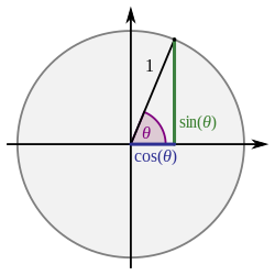


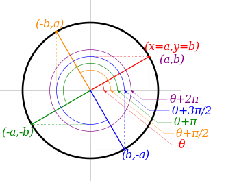


![{\displaystyle {\begin{aligned}\operatorname {sgn}(\sin \theta )=\operatorname {sgn}(\csc \theta )&={\begin{cases}+1&{\text{if}}\ \ 0<\theta <\pi \\-1&{\text{if}}\ \ {-\pi }<\theta <0\\0&{\text{if}}\ \ \theta \in \{0,\pi \}\end{cases}}\\[5mu]\operatorname {sgn}(\cos \theta )=\operatorname {sgn}(\sec \theta )&={\begin{cases}+1&{\text{if}}\ \ {-{\tfrac {1}{2}}\pi }<\theta <{\tfrac {1}{2}}\pi \\-1&{\text{if}}\ \ {-\pi }<\theta <-{\tfrac {1}{2}}\pi \ \ {\text{or}}\ \ {\tfrac {1}{2}}\pi <\theta <\pi \\0&{\text{if}}\ \ \theta \in {\bigl \{}{-{\tfrac {1}{2}}\pi },{\tfrac {1}{2}}\pi {\bigr \}}\end{cases}}\\[5mu]\operatorname {sgn}(\tan \theta )=\operatorname {sgn}(\cot \theta )&={\begin{cases}+1&{\text{if}}\ \ {-\pi }<\theta <-{\tfrac {1}{2}}\pi \ \ {\text{or}}\ \ 0<\theta <{\tfrac {1}{2}}\pi \\-1&{\text{if}}\ \ {-{\tfrac {1}{2}}\pi }<\theta <0\ \ {\text{or}}\ \ {\tfrac {1}{2}}\pi <\theta <\pi \\0&{\text{if}}\ \ \theta \in {\bigl \{}{-{\tfrac {1}{2}}\pi },0,{\tfrac {1}{2}}\pi ,\pi {\bigr \}}\end{cases}}\end{aligned}}}](https://wikimedia.org/api/rest_v1/media/math/render/svg/14cc79239a0fcdfb53b132d75a93474e9e6d5ba0)

![{\displaystyle ({-\pi },\pi ],}](https://wikimedia.org/api/rest_v1/media/math/render/svg/122328145a5f3a4162d21b4fbb5f4d1149932d2b)


![{\displaystyle {\begin{aligned}e_{0}&=1\\[6pt]e_{1}&=\sum _{i}x_{i}&&=\sum _{i}\tan \theta _{i}\\[6pt]e_{2}&=\sum _{i<j}x_{i}x_{j}&&=\sum _{i<j}\tan \theta _{i}\tan \theta _{j}\\[6pt]e_{3}&=\sum _{i<j<k}x_{i}x_{j}x_{k}&&=\sum _{i<j<k}\tan \theta _{i}\tan \theta _{j}\tan \theta _{k}\\&\ \ \vdots &&\ \ \vdots \end{aligned}}}](https://wikimedia.org/api/rest_v1/media/math/render/svg/cb1927ae2be96f5156e18813a20486fdb0ff72f1)
![{\displaystyle {\begin{aligned}{\tan }{\Bigl (}\sum _{i}\theta _{i}{\Bigr )}&={\frac {{\sin }{\bigl (}\sum _{i}\theta _{i}{\bigr )}/\prod _{i}\cos \theta _{i}}{{\cos }{\bigl (}\sum _{i}\theta _{i}{\bigr )}/\prod _{i}\cos \theta _{i}}}\\[10pt]&={\frac {\displaystyle \sum _{{\text{odd}}\ k\geq 1}(-1)^{\frac {k-1}{2}}\sum _{\begin{smallmatrix}A\subseteq \{1,2,3,\dots \}\\\left|A\right|=k\end{smallmatrix}}\prod _{i\in A}\tan \theta _{i}}{\displaystyle \sum _{{\text{even}}\ k\geq 0}~(-1)^{\frac {k}{2}}~~\sum _{\begin{smallmatrix}A\subseteq \{1,2,3,\dots \}\\\left|A\right|=k\end{smallmatrix}}\prod _{i\in A}\tan \theta _{i}}}={\frac {e_{1}-e_{3}+e_{5}-\cdots }{e_{0}-e_{2}+e_{4}-\cdots }}\\[10pt]{\cot }{\Bigl (}\sum _{i}\theta _{i}{\Bigr )}&={\frac {e_{0}-e_{2}+e_{4}-\cdots }{e_{1}-e_{3}+e_{5}-\cdots }}\end{aligned}}}](https://wikimedia.org/api/rest_v1/media/math/render/svg/d02567417a5a013481366384787e518cd74c68be)
![{\displaystyle {\begin{aligned}\tan(\theta _{1}+\theta _{2})&={\frac {e_{1}}{e_{0}-e_{2}}}={\frac {x_{1}+x_{2}}{1\ -\ x_{1}x_{2}}}={\frac {\tan \theta _{1}+\tan \theta _{2}}{1\ -\ \tan \theta _{1}\tan \theta _{2}}},\\[8pt]\tan(\theta _{1}+\theta _{2}+\theta _{3})&={\frac {e_{1}-e_{3}}{e_{0}-e_{2}}}={\frac {(x_{1}+x_{2}+x_{3})\ -\ (x_{1}x_{2}x_{3})}{1\ -\ (x_{1}x_{2}+x_{1}x_{3}+x_{2}x_{3})}},\\[8pt]\tan(\theta _{1}+\theta _{2}+\theta _{3}+\theta _{4})&={\frac {e_{1}-e_{3}}{e_{0}-e_{2}+e_{4}}}\\[8pt]&={\frac {(x_{1}+x_{2}+x_{3}+x_{4})\ -\ (x_{1}x_{2}x_{3}+x_{1}x_{2}x_{4}+x_{1}x_{3}x_{4}+x_{2}x_{3}x_{4})}{1\ -\ (x_{1}x_{2}+x_{1}x_{3}+x_{1}x_{4}+x_{2}x_{3}+x_{2}x_{4}+x_{3}x_{4})\ +\ (x_{1}x_{2}x_{3}x_{4})}},\end{aligned}}}](https://wikimedia.org/api/rest_v1/media/math/render/svg/4c9196b8ab5e0aef6cf7d7fec7d7546f2a6e7d2f)
![{\displaystyle {\begin{aligned}{\sec }{\Bigl (}\sum _{i}\theta _{i}{\Bigr )}&={\frac {\prod _{i}\sec \theta _{i}}{e_{0}-e_{2}+e_{4}-\cdots }}\\[8pt]{\csc }{\Bigl (}\sum _{i}\theta _{i}{\Bigr )}&={\frac {\prod _{i}\sec \theta _{i}}{e_{1}-e_{3}+e_{5}-\cdots }}\end{aligned}}}](https://wikimedia.org/api/rest_v1/media/math/render/svg/b24f2b169fbe11608507c63f5bb728e03b2b4957)


![{\displaystyle {\begin{aligned}\sec(\alpha +\beta +\gamma )&={\frac {\sec \alpha \sec \beta \sec \gamma }{1-\tan \alpha \tan \beta -\tan \alpha \tan \gamma -\tan \beta \tan \gamma }}\\[8pt]\csc(\alpha +\beta +\gamma )&={\frac {\sec \alpha \sec \beta \sec \gamma }{\tan \alpha +\tan \beta +\tan \gamma -\tan \alpha \tan \beta \tan \gamma }}.\end{aligned}}}](https://wikimedia.org/api/rest_v1/media/math/render/svg/e082e69aab7a9c782f590f3a93262ba3101899b7)
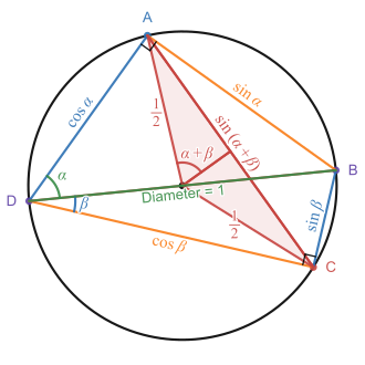


![{\displaystyle {\begin{aligned}\sin {\frac {\theta }{2}}&=\operatorname {sgn} \left(\sin {\frac {\theta }{2}}\right){\sqrt {\frac {1-\cos \theta }{2}}}\\[3pt]\cos {\frac {\theta }{2}}&=\operatorname {sgn} \left(\cos {\frac {\theta }{2}}\right){\sqrt {\frac {1+\cos \theta }{2}}}\\[3pt]\tan {\frac {\theta }{2}}&={\frac {1-\cos \theta }{\sin \theta }}={\frac {\sin \theta }{1+\cos \theta }}=\csc \theta -\cot \theta ={\frac {\tan \theta }{1+\sec {\theta }}}\\[6mu]&=\operatorname {sgn}(\sin \theta ){\sqrt {\frac {1-\cos \theta }{1+\cos \theta }}}={\frac {-1+\operatorname {sgn}(\cos \theta ){\sqrt {1+\tan ^{2}\theta }}}{\tan \theta }}\\[3pt]\cot {\frac {\theta }{2}}&={\frac {1+\cos \theta }{\sin \theta }}={\frac {\sin \theta }{1-\cos \theta }}=\csc \theta +\cot \theta =\operatorname {sgn}(\sin \theta ){\sqrt {\frac {1+\cos \theta }{1-\cos \theta }}}\\\sec {\frac {\theta }{2}}&=\operatorname {sgn} \left(\cos {\frac {\theta }{2}}\right){\sqrt {\frac {2}{1+\cos \theta }}}\\\csc {\frac {\theta }{2}}&=\operatorname {sgn} \left(\sin {\frac {\theta }{2}}\right){\sqrt {\frac {2}{1-\cos \theta }}}\\\end{aligned}}}](https://wikimedia.org/api/rest_v1/media/math/render/svg/d53d104c73c4b28f1dd7bfa5d2b0c7207c68cd87)
![{\displaystyle {\begin{aligned}\tan {\frac {\eta \pm \theta }{2}}&={\frac {\sin \eta \pm \sin \theta }{\cos \eta +\cos \theta }}\\[3pt]\tan \left({\frac {\theta }{2}}+{\frac {\pi }{4}}\right)&=\sec \theta +\tan \theta \\[3pt]{\sqrt {\frac {1-\sin \theta }{1+\sin \theta }}}&={\frac {\left|1-\tan {\frac {\theta }{2}}\right|}{\left|1+\tan {\frac {\theta }{2}}\right|}}\end{aligned}}}](https://wikimedia.org/api/rest_v1/media/math/render/svg/639270245e163f1afa8682ac8aa12086db43dce1)


![{\displaystyle {\begin{aligned}\tan {\frac {\theta }{2}}&=\csc \theta -\cot \theta \\&=\pm \,{\sqrt {\frac {1-\cos \theta }{1+\cos \theta }}}\\[3pt]&={\frac {\sin \theta }{1+\cos \theta }}\\[3pt]&={\frac {1-\cos \theta }{\sin \theta }}\\[5pt]\tan {\frac {\eta +\theta }{2}}&={\frac {\sin \eta +\sin \theta }{\cos \eta +\cos \theta }}\\[5pt]\tan \left({\frac {\theta }{2}}+{\frac {\pi }{4}}\right)&=\sec \theta +\tan \theta \\[5pt]{\sqrt {\frac {1-\sin \theta }{1+\sin \theta }}}&={\frac {\left|1-\tan {\frac {\theta }{2}}\right|}{\left|1+\tan {\frac {\theta }{2}}\right|}}\\[5pt]\tan {\frac {\theta }{2}}&={\frac {\tan \theta }{1+{\sqrt {1+\tan ^{2}\theta }}}}\\&{\text{for }}\theta \in \left(-{\tfrac {\pi }{2}},{\tfrac {\pi }{2}}\right)\end{aligned}}}](https://wikimedia.org/api/rest_v1/media/math/render/svg/3cab50a58d64b8c3341fb4f7646888bbbc67ea0c)
![{\displaystyle {\begin{aligned}\cot {\frac {\theta }{2}}&=\csc \theta +\cot \theta \\&=\pm \,{\sqrt {\frac {1+\cos \theta }{1-\cos \theta }}}\\[3pt]&={\frac {\sin \theta }{1-\cos \theta }}\\[4pt]&={\frac {1+\cos \theta }{\sin \theta }}\end{aligned}}}](https://wikimedia.org/api/rest_v1/media/math/render/svg/5c9be831a310f112ffc6e5790bc705dc7b070b87)


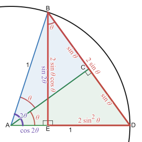


![{\displaystyle {\begin{aligned}\prod _{k=1}^{n}\cos \theta _{k}&={\frac {1}{2^{n}}}\sum _{e\in S}\cos(e_{1}\theta _{1}+\cdots +e_{n}\theta _{n})\\[6pt]&{\text{where }}e=(e_{1},\ldots ,e_{n})\in S=\{1,-1\}^{n}\end{aligned}}}](https://wikimedia.org/api/rest_v1/media/math/render/svg/ce2126a8ded0d0c92cf2bc4e9386c34430513c4b)


![{\displaystyle {\begin{aligned}\sum _{k=0}^{n}\sin k\theta &={\frac {\cos {\tfrac {1}{2}}\theta -\cos \left(\left(n+{\tfrac {1}{2}}\right)\theta \right)}{2\sin {\tfrac {1}{2}}\theta }}\\[5pt]\sum _{k=0}^{n}\cos k\theta &={\frac {\sin {\tfrac {1}{2}}\theta +\sin \left(\left(n+{\tfrac {1}{2}}\right)\theta \right)}{2\sin {\tfrac {1}{2}}\theta }}\end{aligned}}}](https://wikimedia.org/api/rest_v1/media/math/render/svg/c850aa2dd7cc306d87d5d68d5802cab64f8572a0)


![{\displaystyle {\begin{aligned}\sin x&=x\prod _{n=1}^{\infty }\left(1-{\frac {x^{2}}{\pi ^{2}n^{2}}}\right),&\cos x&=\prod _{n=1}^{\infty }\left(1-{\frac {x^{2}}{\pi ^{2}\left(n-{\frac {1}{2}}\right)\!{\vphantom {)}}^{2}}}\right),\\[10mu]\sinh x&=x\prod _{n=1}^{\infty }\left(1+{\frac {x^{2}}{\pi ^{2}n^{2}}}\right),&\cosh x&=\prod _{n=1}^{\infty }\left(1+{\frac {x^{2}}{\pi ^{2}\left(n-{\frac {1}{2}}\right)\!{\vphantom {)}}^{2}}}\right).\end{aligned}}}](https://wikimedia.org/api/rest_v1/media/math/render/svg/6d43e1176a38b1e6b653837eb782ae79735783ac)


![{\displaystyle {\begin{alignedat}{9}{\frac {\pi }{2}}~&=~\arcsin(x)&&+\arccos(x)~&&=~\arctan(r)&&+\operatorname {arccot}(r)~&&=~\operatorname {arcsec}(s)&&+\operatorname {arccsc}(s)\\[0.4ex]\pi ~&=~\arccos(x)&&+\arccos(-x)~&&=~\operatorname {arccot}(r)&&+\operatorname {arccot}(-r)~&&=~\operatorname {arcsec}(s)&&+\operatorname {arcsec}(-s)\\[0.4ex]0~&=~\arcsin(x)&&+\arcsin(-x)~&&=~\arctan(r)&&+\arctan(-r)~&&=~\operatorname {arccsc}(s)&&+\operatorname {arccsc}(-s)\\[1.0ex]\end{alignedat}}}](https://wikimedia.org/api/rest_v1/media/math/render/svg/839db041f421b4af5890106450e2b4d3e9e183d4)


